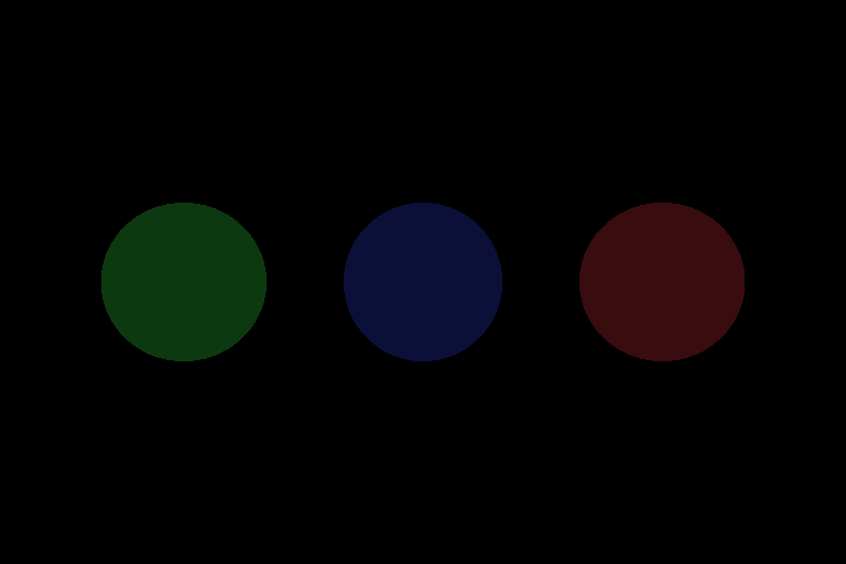
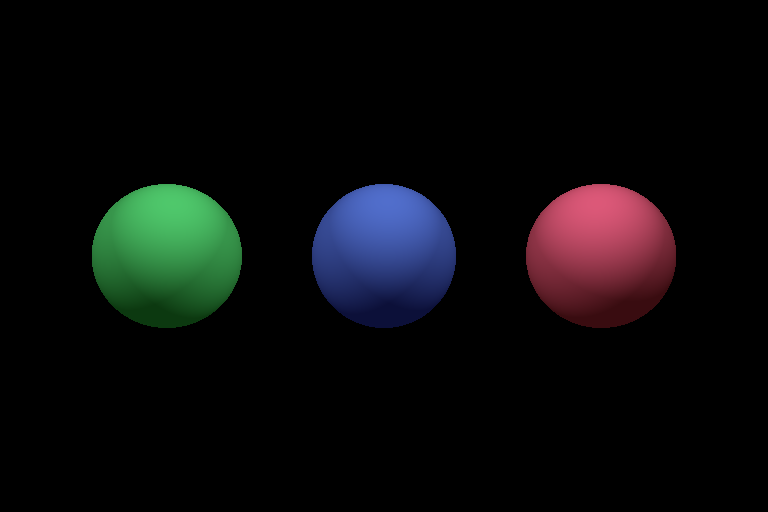
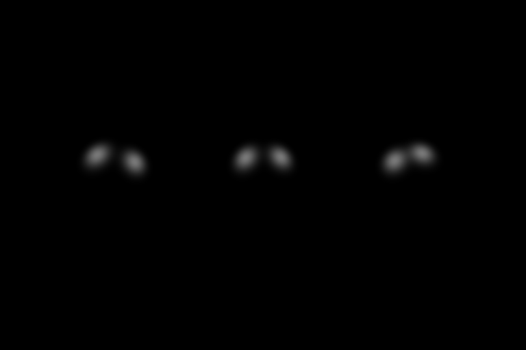
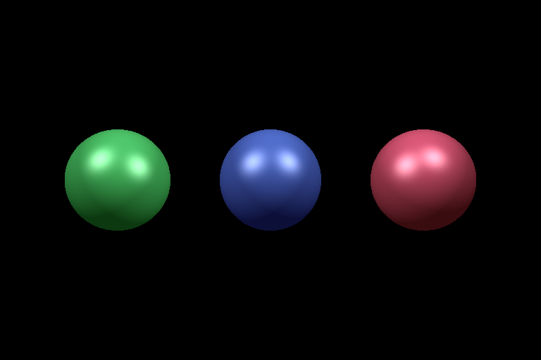
Lab 6: Light

Github Classroom assignment

Please put your answers to written questions in this lab, if any, in a Markdown file named README.md in your lab repo.

Introduction

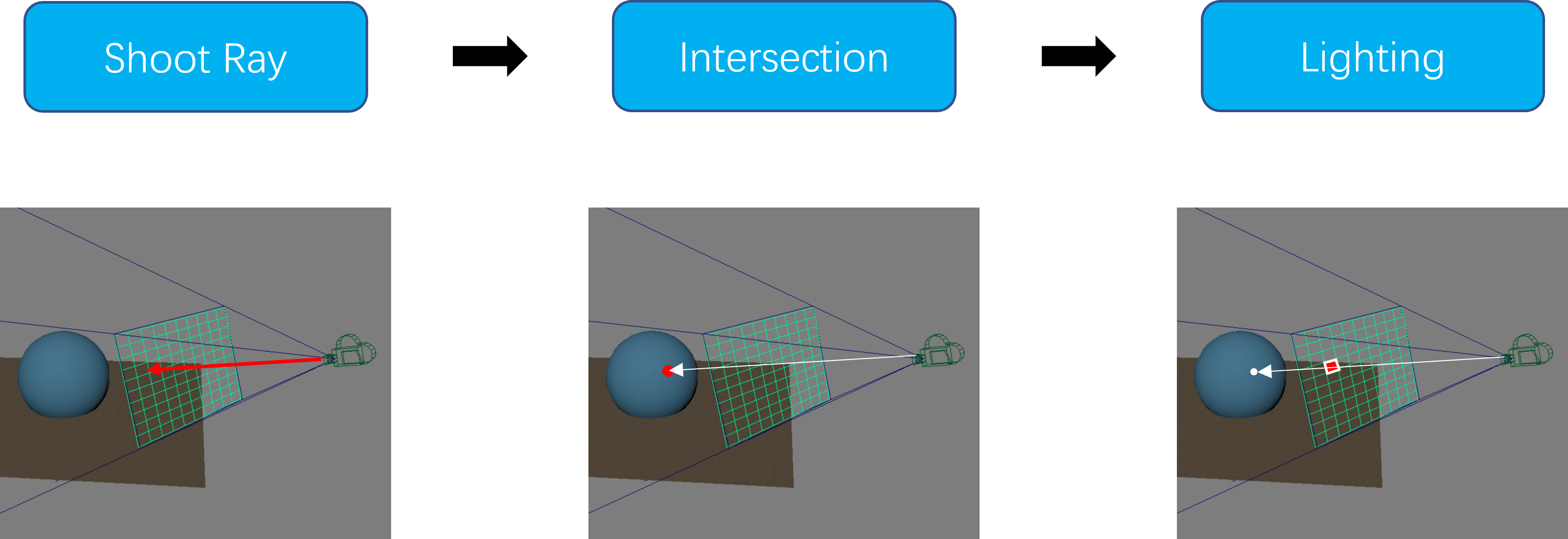
If you've started Project 3: Intersect, you might already have implemented the first two parts of the raytracing pipeline—ray generation and object intersection.

This is, of course, not our end goal. What we really want is for our raytracers to be able to produce realistic images, which would require rethinking how we assign colors to pixels. To that end, we're going to explore the subject of lighting: what it is, how it works, and how you can implement it.

Objectives

Learn about lighting, especially lighting models,
Implement the Phong lighting model, and
Extend it to implement other lighting effects, like reflection.

Conceptual Context

We will be covering quite a bit of background knowledge in this lab before we can get to any actual tasks. This is important information for both Project 4: Illuminate and Project 6: Action!, which is why we're emphasizing it so heavily. Skim at your own risk!

What Is Lighting?

Lighting is the simulation of how light interacts with objects. It is an essential part of photorealistic rendering—the generation of a physically-plausible image from a scene.

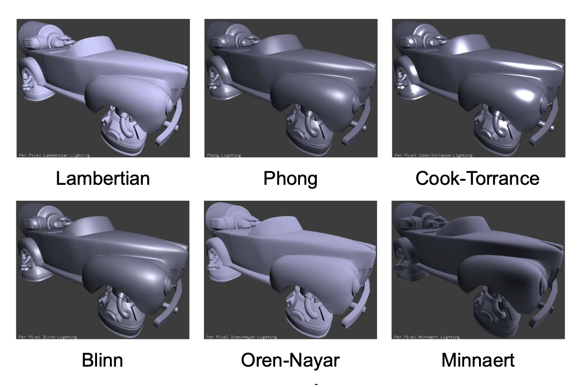
TODO — **Figure 1:** Raytracing is a method of photorealistic rendering. Naturally, it includes a lighting step.

Unfortunately, accurately simulating light is really hard. Instead, we approximate it using simplified lighting models, such as the Phong, Cook-Torrance, Minnaert and Oren-Nayer models.

Each lighting model mathematically describes the interactions between objects' surfaces and light, though they might differ in their underlying physical bases and assumptions.

The Phong Lighting Model

In this lab, and in your raytracer, you will be using the Phong lighting model.

What It Is

The Phong lighting model is represented by an equation which has three main terms—ambient, diffuse, and specular.

Here is a simplified version of that equation:

And here it is again, as an image:

Extra: why do we use this lighting model in particular?

We use the Phong illumination model in CS 1230 because it's conceptually straightforward and fairly easy to implement.

Other models based on more complicated physical phenomena can and do provide more realistic results, but they also tend to require more understanding to get right, as well as more material parameters.

How It Works

The Phong lighting model determines the output color of each pixel in your rendered image based on the following inputs:

The position of and surface normal at the point of intersection,
The material properties of the intersected surface/object,
The placement and properties of light sources in the scene, and
Other adjustable global parameters, such as the weight for each component of the lighting model.

This output color is effectively the simulated intensity of the "light" traveling along a "ray" from the intersection point to the camera.

But I thought rays shot out from the camera, not towards it!

It actually doesn't matter which direction you imagine rays "travel", since they're fairly reversible. We usually adopt the view that's most convenient for our use case:

When thinking about light travelling from a light source, hitting a surface, and bouncing towards a camera, it makes more sense to think about the decreasing amount of light as it travels from source to destination. Physically speaking, this interpretation is "more correct".

When generating rays, we have to pretend that those rays shoot out from the camera. Otherwise, if we instead generated rays starting from light sources, we'd have to generate infinitely many rays and check each one to see they reach our infinitesimally small camera. Needless to say, this is not at all efficient.

Given this, it may seem like raytracing is "backwards". Well... it sort of is!

Further reading: forward and backward raytracing, bidirectional path tracing.

Task Context

In this lab, you will complete a single function which implements Phong lighting: it will produce an output RGBA color, given some input data.

The above function can be found in lightmodel.cpp. This is the only file you have to modify.

That said, we strongly recommend that you at least take a look at the rest of the stencil, particularly param.h and main.cpp. The former declares global parameters (discussed in a later section), along with some of the data structures you'll be working with, and the latter gives you a broader-picture understanding of what you're implementing.

It's Always Arrays

In order to focus solely on the lighting part of raytracing, you will not have to generate rays and obtain intersections. We will provide you with all the necessary data, e.g. intersection position, surface normals, and global parameters.

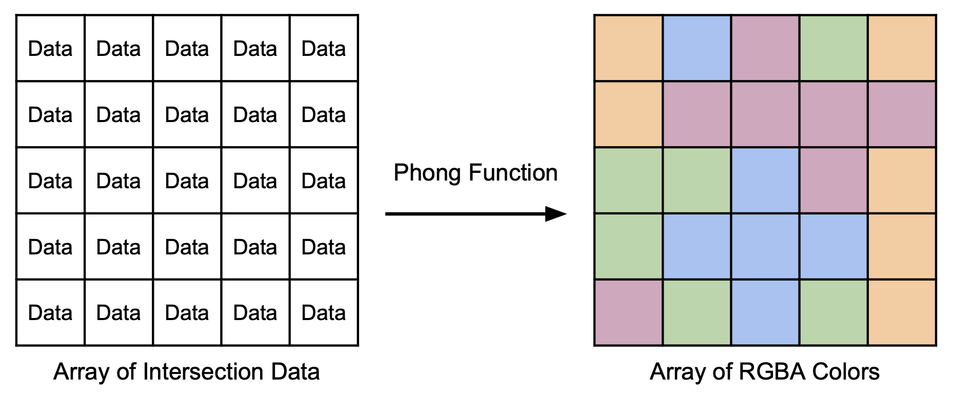
This data will come in the form of a 2D array of structs (each containing the necessary data) with height and width equal to the final image we're expecting.

Your function will work at the pixel level, and you will use it to map every element in this array to an output RGBA color.

Spoiler: About the program you're writing...

This function is technically a shader program. A shader computes the color of each pixel with given per-pixel data. You'll get to learn more about shaders in lab 10, and you'll use them in Project 6: Action!.

Global Parameters

On top of this array of data, you'll also need some additional global parameters (e.g. weights for lighting model components, and the positions of light sources).

These, too, will be provided to your function in the form of global variables in param.h:

float ka;  // weight for ambient light
float kd;  // weight for diffuse light
float ks;  // weight for specular light
float kr;  // weight for mirror reflection
float c1;  // attenuation coefficient 1
float c2;  // attenuation coefficient 2
float c3;  // attenuation coefficient 3

A Note On Light Sources

In Project 4: Illuminate, you will be required to support point lights, directional lights, and spotlights. You will also have to implement shadows.

In this lab, however, you will work only with point lights, and you will not have to implement shadows.

As a reminder, point lights are sources which emit light uniformly in all directions from a single position.

Clamping

One last thing!

As you already know, we display our images using the RGBA color format, which is a tuple of four integers, bounded in the range [0,255].

However, there is no bound on the color intensity we might obtain from the Phong lighting equation (below), i.e. we could get a value anywhere from zero to infinity.

Thus, we must map our output color values to something between 0 and 255. Though there are many other ways to do this, here, we've chosen the simplest: clamping our output values to the range [0,x], then scaling them linearly to [0,255]. Purely based on our coefficient selection, it happens that x = 1 is a good choice for this purpose.

In the helper function at src/lightmodel.cpp, implement the above clamping operation. This helper function will take in a glm::vec4 of float values and return a single RGBA struct.

You can leave the alpha value of the RGBA struct at its default (255)

Extra: we mentioned "other ways to do this". What is "this"?

"... we must map our output intensity values ..."

"This" refers to tone-mapping.

It describes the mapping of wider set of intensities/colors into a narrower set. Tone-mapping is typically done to convert high dynamic range (HDR) images to more limited-range, 24-bit RGB formats like JPEG or PNG, while approximating the appearance of HDR.

Tone mapping is crucial to computer graphics as most rendering methods produce intensity values with high dynamic ranges. In fact, it is even crucial to real-world photography, since there is no (meaningful) bound on light intensity out there, either!

Extra: we mentioned "other ways to do this". What are these other ways?

Many different methods of tone-mapping exist, each producing images with unique visual effects.

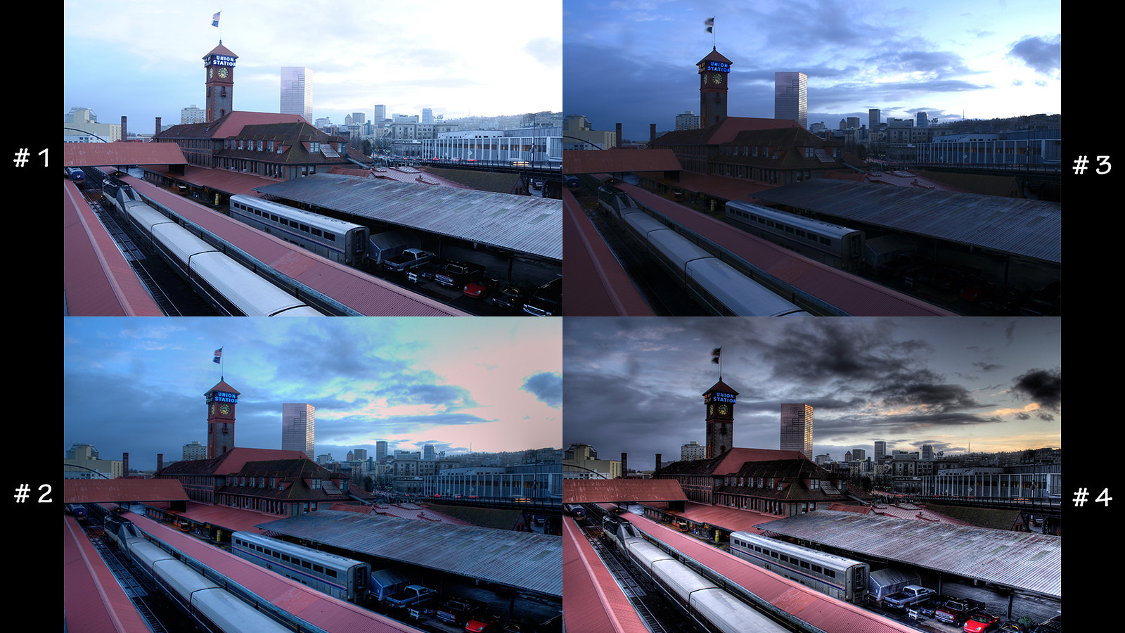
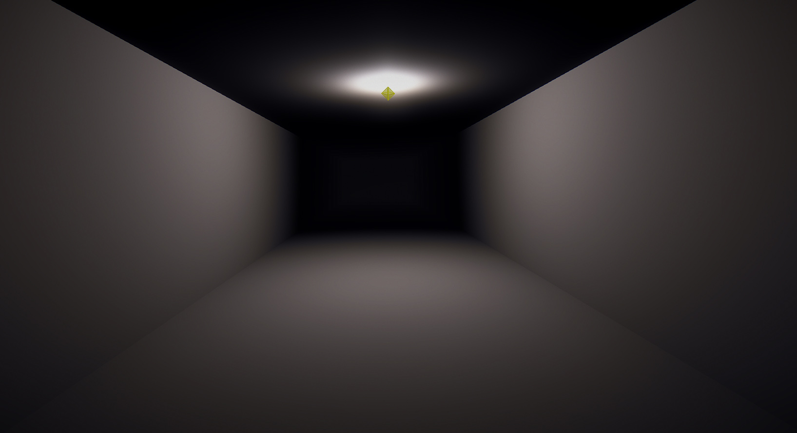
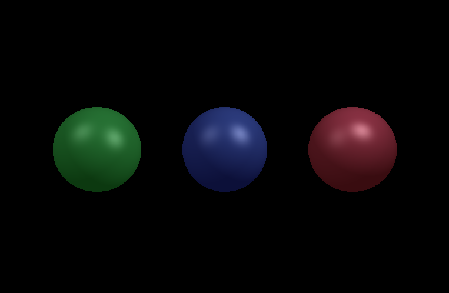
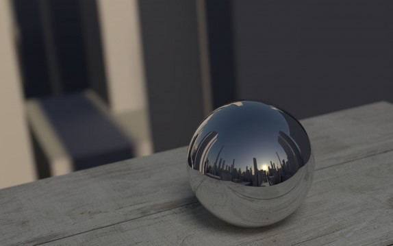
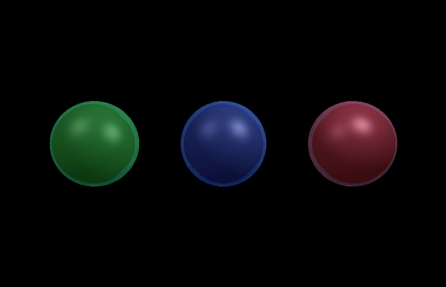
Mapping can either be globally-consistent across the whole image (e.g. uniform scaling), or be locally-adaptive, so that overly-bright and overly-dark areas can be shown with minimal loss of detail. Images #3 and #4 below show how a locally-adaptive form of tone-mapping can improve the visual clarity of the final image.

The method of tone-mapping we chose, clamping, is extremely naïve: it will cause us to lose information in areas with strong illumination. But, it is very simple, stable, and effective enough for the scope of this lab—if you are interested, you will have the chance to discover more tone mapping techniques later in this course.

Implementing The Phong Lighting Model

Remember this simplified version of the Phong lighting equation?

Here it is in full!

This is one of the most important equations you'll learn in CS 1230. You are not really expected to understand this in full right now, but you will know it like the back of your hand by the end of this course. For now, simply bask in its glory (and complete the next task).

A very detailed breakdown of each symbol in the equation is available in the collapsible section below. Using this as reference, answer the following questions:

Supposing that you wish to output a single RGB color, how many times would you need to perform the above calculation for a given intersection point?
How many distinct, scalar-valued material parameters are necessary for the above RGB color computation(s)? Please list all of them.

Jot these down for your lab checkoff later.

Click here for a full breakdown of the equation's terms.

Subscript	What It Represents
	A given wavelength (either red, green, or blue).
/ /	A given component of the Phong illumination model (either ambient, diffuse, or specular).
	A given light source, one of lights in the scene.

Symbol	What It Represents
	The intensity of light. E.g. would represent the intensity of red light, and is the intensity of blue light for a given light with index .
	A model parameter used to tweak the relative weights of the Phong lighting model's three terms. E.g. would represent the ambient coefficient.
	A material property, which you can think of as the material's "amount of color" for a given illumination component. E.g. represents how red the material is, when counting only ambient illumination.
	The total number of light sources in the scene.
	The surface normal at the point of intersection.
	The normalized direction from the intersection point to light .
	The reflected light of about normal .
	The normalized direction from the intersection point to the camera.
	A different material property. This one's called the specular exponent or shininess, and a surface with a higher shininess value will have a narrower specular highlight, i.e. a light reflected on its surface will appear more focused.
	The attenuation factor. More on this later.

The Ambient Term

The first thing to do in implementing Phong lighting will be to add in the ambient term. This simply adds some uniform amount of light to everything in the scene, independent of light sources. It is used to fake the effect of indirect lighting, so as to avoid having to perform expensive simulations of indirect light from rays which bounce multiple times.

In your Phong lighting function, add the ambient term to the return value. Refer to the equation above.

The Diffuse Term

Next, we'll add the diffuse term to make surfaces facing light sources appear brighter. This emulates the real-world phenomenon of Lambertian reflectance (aka ideal diffuse reflection), wherein a surface scatters incident photons uniformly across the hemisphere centered on its normal.

To quantify how much a surface is facing a light source, we use the dot product , where is the surface normal at the point of intersection and is the normalized direction from the intersection point to the light source.

If a surface is facing away from a light source, it should not be lit by that light source, i.e. it should add zero (not negative!) intensity to the result.

In your Phong lighting function, add the diffuse term to the return value. Refer to the equation above.

For now, ignore attenuation (set to 1).
Make sure to normalize all your directions.
Consider how you might determine if a surface is facing away from a light source.
Remember that you have to sum over all the lights in the scene.

Extra: what do the sub-terms in the diffuse term mean?

Ignoring attenuation, there is first the product of light intensity, the diffuse coefficient, and the material's diffuse color. This should be easily understood.

Besides that, there is also the dot product .

This is based on Lambert's cosine law. It was Johann Heinrich Lambert who first introduced the concept of perfect diffusion in his 1760 book on optics, Photometria. He had observed that most flat, rough surfaces would reflect light in a way roughly proportional to the cosine of the angle between their surface normal and the direction toward the incoming light.

Fortunately for us, we can easily and efficiently compute cosines using a dot product of normalized vectors. Thus, by using the dot product above, we can suggest diffuse reflectance.

On finishing this task, you should be able to see the image below.

The Specular Term

Specular, adj.
Relating to or having the properties of a mirror.

Our third step is to add the specular term, which creates a specular highlight that makes objects appear shiny or mirror-like. This approximates the specular reflection of incident light, which peaks in intensity when the reflected light is "close" to the direction of the eye. Again, we use a dot product, , to quantify this "close"-ness.

here is the reflected direction of incoming light about surface normal, and should be the direction to the camera. Both are pointing away from the intersection point.

In order to make this specular highlight wider or narrower, we can lower or raise the exponent , which represents the material's shininess. The higher the exponent, the smaller the highlight, and the more mirror-like the resulting surface.

In your Phong lighting function, add the specular term to the return value. Refer to the equation above.

Again, ignore attenuation (set to 1).
Make sure to normalize all your directions.
Remember to consider the case of a surface facing away from a light source.
Remember that you have to sum over all the lights in the scene.

You will have to calculate reflections in this and later tasks. We suggest that you calculate these by hand, and be aware of which way each vector you're using is pointing.

You may use built-in glm functions. However, it will be on you to make sure you get the interfaces right.

On finishing this task, you should be able to see the image below.

Attenuation

Finally, we get to the attenuation factor. In the real world, the intensity of light is usually diminished with increasing distance from light source (with the notable exception of collimated light, i.e. ideal lasers). For example, the intensity of a point source's light is scaled by a factor of at distance from the source, due to the dispersal of energy over an expanding surface.

This is demonstrated in the image below: the objects farthest from the light source are noticeably darker than those closest to it. This effect is not entirely attributable to the differences in angles formed by the light directions, camera directions, and surface normals (refer back to the diffuse and specular terms).

Modify your Phong lighting function to account for attenuation. Use the following, generalized substitution:

Experiment by changing , , and . How does this affect the render?

On finishing this task, you should be able to see the image below (using the default , , and values).

Reflection

We can extend the Phong illumination model by adding some other components to make the image look even better.

One interesting and simple extension is mirror reflection, as in the figure below:

We can achieve reflection via recursive raytracing: at each intersection with a reflective surface, we can perform raytracing again from that intersection point in the reflected direction. We then add the color returned by that recursive call to the color of our intersection point, scaled by a reflective material parameter :

When you implement your fully-fledged raytracer, you will simulate multiple recursive light bounces using this method. For this lab, you'll implement a simpler version, with:

Only once bounce of mirror reflection, and
No actual recursive call to your full raytracing function—instead, we provide a function that tells you what the reflected illumination would be if you were to actually trace the ray.

We've provided you with a function getReflection(source, dir) to acquire the reflected illumination for a ray starting at source in the direction dir. We've also called this function for you according to the equation above.

However, we've incorrectly computed the reflected ray direction, resulting in incorrect reflected illumination values.

Uncomment the lines before the return statement of phong() and run the code; the output shouldn't look quite right compared to the ground truth (it should currently match Figure 15)

buggy provided reflections — **Figure 16:** Provided buggy reflections

**Figure 17:** Expected correct reflections. Final Result.

Fix the calculation of reflectedDirection!
Verify that your output matches Figure 16 above. Be prepared to briefly explain what the bug is and how you found it during your checkoff.

Hint:

Recall from lecture 9 that the formula for reflecting an incoming ray direction about a surface normal is

Pay special attention to the orientations of these quantities.

You are not allowed to use glm::reflect() for this debugging exercise!

To help you debug, we recommend drawing an example and applying the reflection formula step-by-step geometrically.

End

Congrats on finishing the Lighting lab! Now, it's time to submit your code and get checked off by a TA.

Submission

Submit your GitHub link and commit ID to the "Lab 6: Light" assignment on Gradescope, then get checked off by a TA at hours.

Reference the GitHub + Gradescope Guide here.