Lab 6: Convolution & Mipmapping
Please put your answers to written questions in this lab, if any, in a Markdown file named README.md in your lab repo.
Introduction
Welcome to Lab 6! This lab is designed to help you get started with Project 4: Antialias.
During this lab, you'll learn about digital image processing (particularly convolution) and mipmapping. The lectures covering this topic can be quite dense, but you can rest assured that the programming you'll be doing is nowhere near as complicated.
Objectives
- Learn about kernels and convolution,
- Begin using convolution to implement more interesting effects, and
- Implement downsampling to generate mipmaps.
Conceptual Background
Broadly, digital image processing is the processing of images through algorithms in order to modify, enhance, or extract useful information from them. These cover a wide range of applications, including noise removal, feature extraction, image compression, and image enhancement.
In this lab, we'll get to explore convolution and mipmapping! Before we get into that, though, here is some optional information which might help contextualize what was taught in lecture:
Digital image processing as signal processing
In lecture, you might've heard about how digital image processing is really just a form of signal processing. This is because a digital image can be seen as a discrete 2D signal—specifically, one which maps a 2D coordinate to a value which tells us the color of the image at that point.
What exactly constitutes a signal is not something we can easily get into here. If you're interested to find out more, do your own research, approach a TA, or ask the professor!
Spatial domain vs. frequency domain
In lecture, you might also have heard about the "spatial" and "frequency" domains. Let's recap:
Mathematically, an image can be described by the function
Since our input to
What other representations can there be? Well,
Confused? Don't worry:
In this lab, we will only be working in the spatial domain.
That said, simply knowing that you can think about images (i.e. signals) in the frequency domain can be quite valuable for a deeper understanding of certain phenomena or effects, such as aliasing, ringing artifacts, and, of course, convolution.
Getting Started
GUI Elements
If you haven't done so, accept the Github Classroom assignment, clone the generated repository, and run the application in Qt Creator. A window that looks like this should appear:
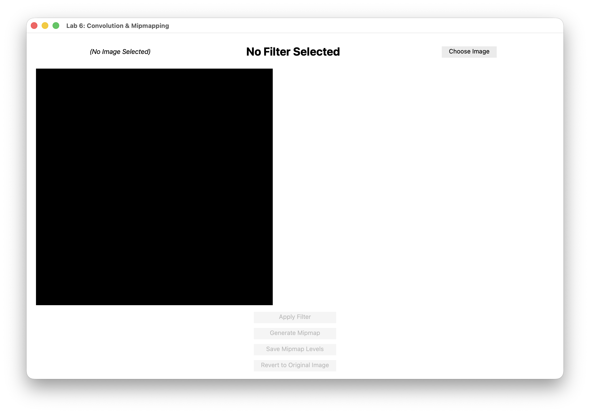
These buttons are fairly self-explanatory, but we'll go through them anyway:
- The
Choose Imagebutton allows you to select any image file from your computer to upload to the canvas. We have provided you with some images in theresourcesdirectory. - The
Apply Filterbutton applies the currently-selected filter to the image. Currently, this does nothing because you have neither implemented, nor selected, any filters. - The
Generate Mipmapbutton displays the mipmap chain of your image. Currently, this does nothing because you have not implemented mipmapping yet. (TODO: verify this from student end view) - The
Save Mipmap Levelsbutton saves the mipmap chain to a folder under themipmaps_generated/student_generationsdirectory. This will help with visualizing and debugging, especially forProject 4: Antialias. - The
Revert to Original Imagebutton reverts the image to its original state.
Interested in how GUI elements like these are set up? Feel free to take a look at
mainwindow.handmainwindow.cppin our stencil code!
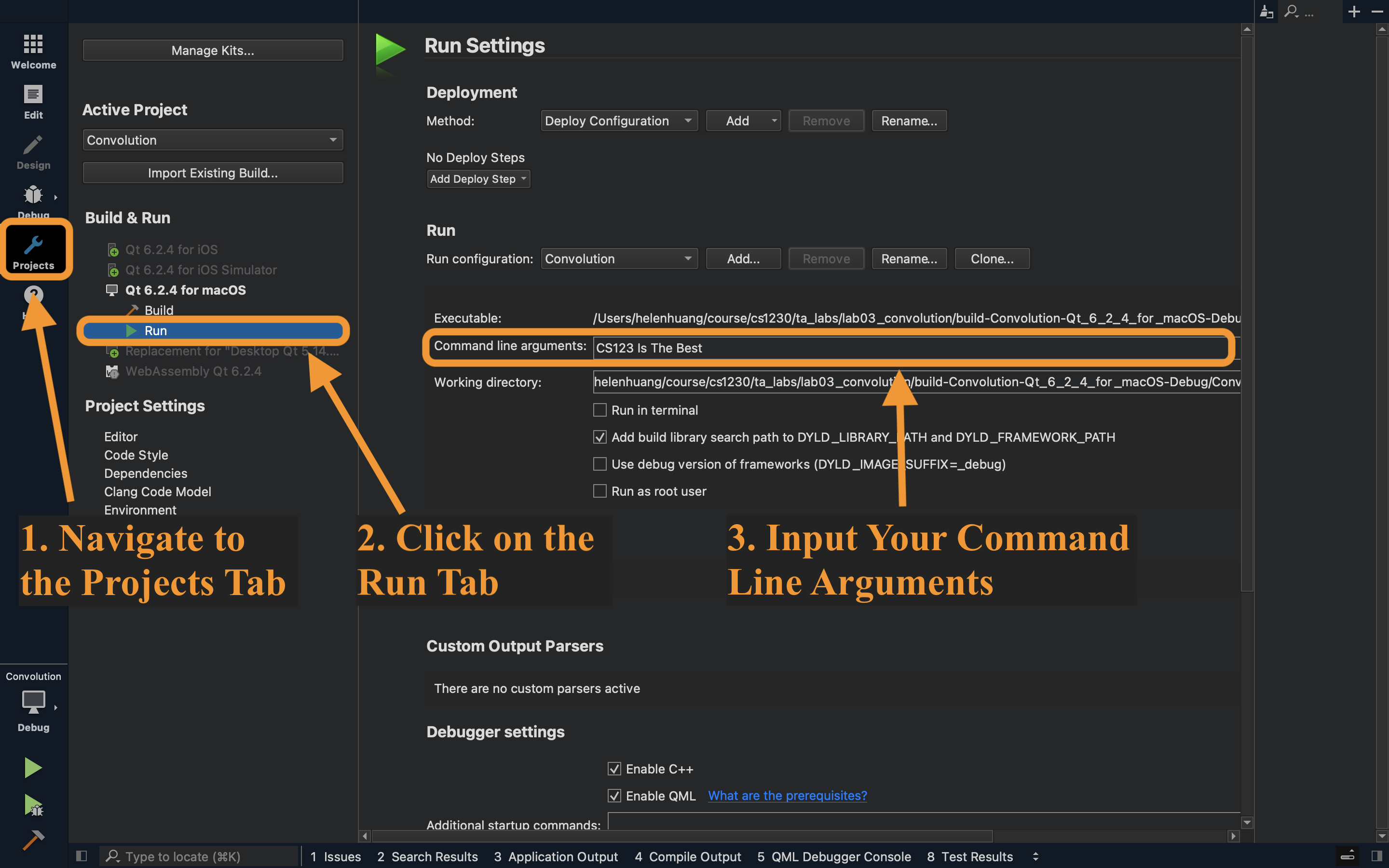
Command Line Arguments
We will use command line arguments to specify the type of the filter we wish to apply to the image. The available filter types are enumerated below.
Filter types (use these as your command line arguments):
identityshiftLeftshiftRight
Reminder: how to set command line arguments
Stencil Code
Take a look through the provided stencil code. In this lab, you will be working with the following files: canvas2d.h, canvas2d.cpp, mipmap.cpp, the files in the filters directory, and settings.h (read-only).
- The
Canvas2Dclass is responsible for storing and manipulating the 2D canvas that will be displayed by the application window. This class has aapplyFilter()method which is called whenever theApply Filterbutton is clicked. - The
mipmap.cppfile is where you will implement the downsampling of the selected image using a separable box filter. - The
filtersdirectory contains severalfilterXYZ.cppfiles, each of which implements afilterXYZ()function. These will be called byapplyFilter()to do specific things, such as shifting the image. The helper functions infilterutilsare used to assist in some of these operations.
Notice that the
filterXYZ()functions are actually methods of theCanvas2Dclass; it's perfectly valid, though less common, to implement functions declared in a.hfile in one or more differently-named.cppfiles.
- The
settingsglobal object contains information about the specific filter type to be applied to the image. You've already seen a similar object used to specify brush settings inProject 1: Brush.
Let's set up the applyFilter() function so that it applies the appropriate filter when the Apply Filter button is clicked.
In applyFilter(), call the appropriate filter functions depending on the filter type, settings.filterType.
settings.filterType is a FilterType enum, which is defined in settings.h. In C++, you can access enum values by writing: EnumName::EnumValue.
- The three filter functions are declared in
canvas2d.h.- From here, you should notice that
filterShift()expects ashiftDirectionargument. This must be aShiftDirectionenum value.
- From here, you should notice that
- We suggest using a
switchstatement to keep your code clean and readable!
Convolution
We will now introduce the concept of convolution, which allows us to apply operations to a pixel while taking into account its neighbors.
Understanding the Process
Generally speaking, convolution is an operation which takes two input signals, and produces an output signal. In digital image processing, we use discrete 2D convolution. This takes in an image and kernel*, and produces an output image.
* A kernel is simply a 2D matrix of values, not unlike an image. And, since convolution is commutative, the distinction between "image" and "kernel" is merely an arbitrary one.
For our purposes, in CS 1230, the steps involved in image convolution as follows:
- Flip/Rotate your kernel
. - Prepare an output image with the same size as your input image.
- For each position in this output image:
- Do an element-wise multiplication between:
- The flipped kernel, and
- The region of the image centered on that position, with the same shape as the flipped kernel.
- Then, compute the sum of the elements of the resulting matrix.
- Finally, set the value of the output image at that position to this sum.
- Do an element-wise multiplication between:
Let's look at an example below.
Worked Example
For simplicity, let us represent our image(s) with only one color channel. In general, convolution is performed per-channel anyway, so this isn't too much of a stretch.
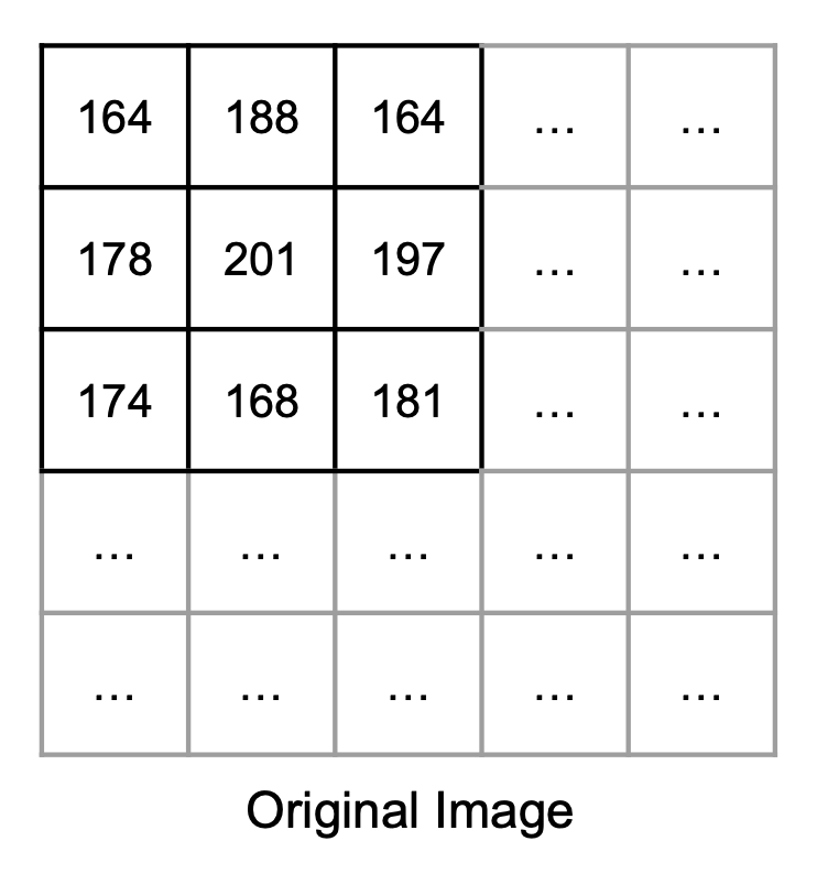
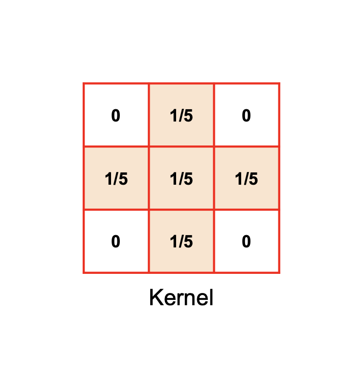
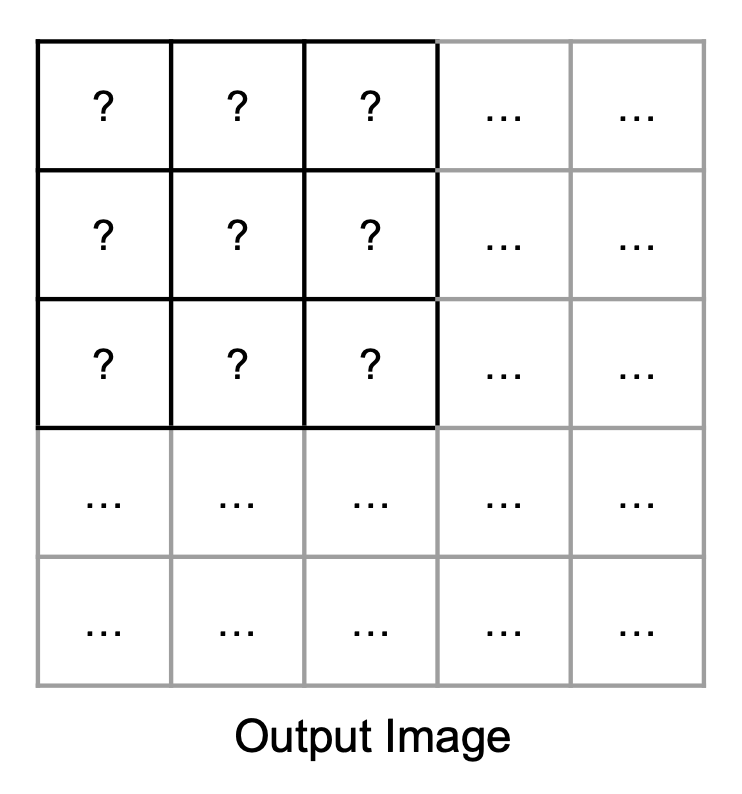
Observe that we are using a normalized kernel, i.e. its sum is Project 4: Antialias.
Also note that, as this kernel is symmetric, it is equal to its flipped self. That means we can make one fewer diagram :)
Next, we can proceed to iterate over every pixel in the output image to determine their values. For this example, we will look only at pixel
As described earlier, a region around the pixel is multiplied element-wise with the kernel, then summed:
Expand for full equation
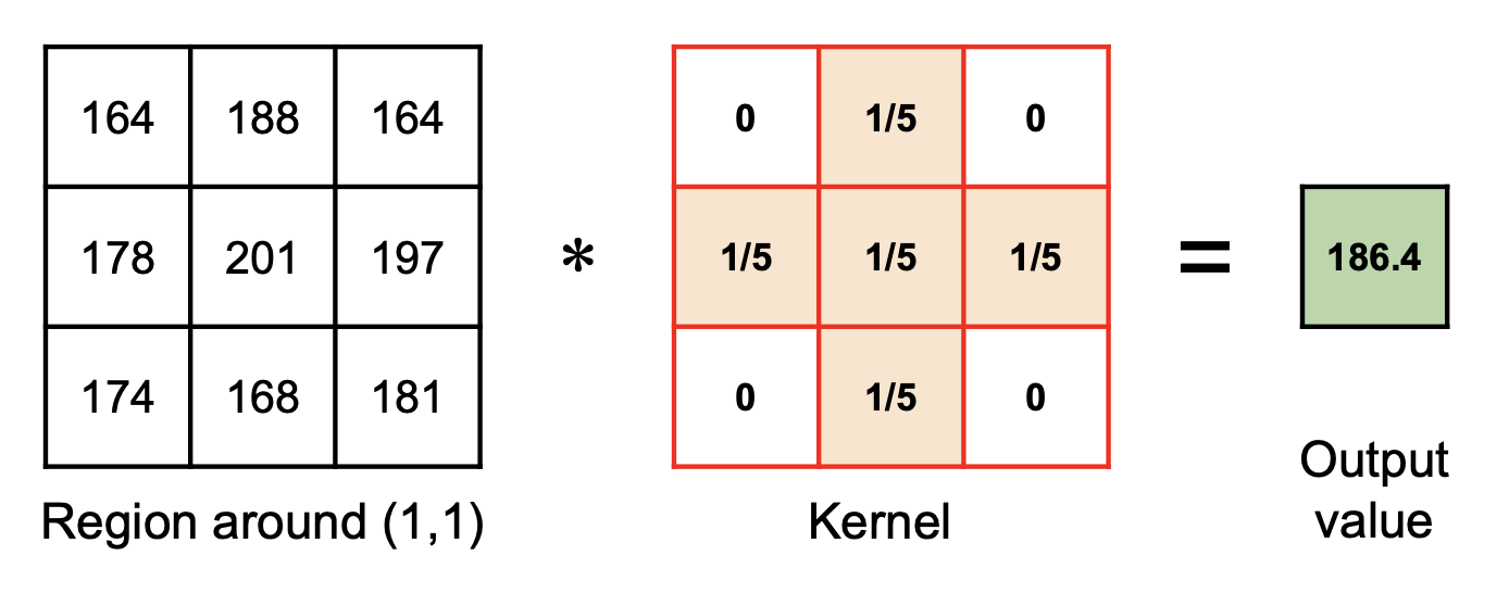
This sum is then stored as the pixel intensity in the output image:
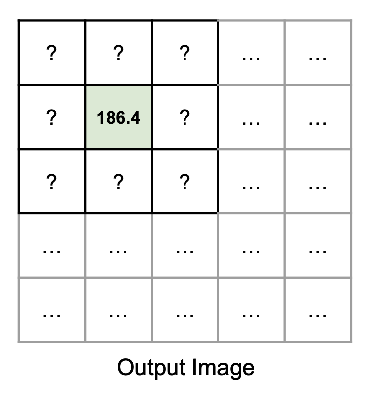
This process of element-wise multiplication and summation must be repeated for every pixel in the output image. As you can probably guess, this makes convolution computationally expensive, due to the large number of multiplications, especially with larger kernels.
If the kernel is separable, then we can reduce computational cost significantly. Given an Project 4: Antialias.
You may be wondering how to perform the above computation for pixels
Implementing Convolution
Finally, let's get to actually implementing the convolve2D() function in filterutils.cpp!
We will follow the steps outlined above, with the caveat that instead of actually flipping our kernel, we'll cleverly index into it "backwards", in a way that effectively flips it. This will be done as part of Task 4.
Preparatory Tasks
First, let's prepare the output image.
In filterutils::convolve2D(), initialize a result RGBA vector to store your output image. This vector should have the same size as your input image, which is stored in data.
Later, in order to perform our element-wise multiplication, we'll need to iterate through the kernel. So, let's also determine the kernel's dimensions.
Obtain the side length of kernel, and store it. You can assume that all kernels are square and have an odd number of rows and columns (so that they have a "center"), at least for this lab.
Beginning The Loop
Now, it's time to implement our element-wise multiplication and sum. This is a pretty big task, so don't be afraid to ask a TA or your peers for help!
- Initialize
redAcc,greenAcc, andblueAccfloat variables to store the accumulated color channels. - Iterate over each element of the kernel, using the kernel dimensions you stored earlier.
- Remember that you must "flip" the kernel.
Tip: The convention for indexing we've been using starts
in the top left corner moving right and down. If we flip the kernel, which corner do we begin and what directions do we move in? This should be a very small change to your code.
- For each iteration, update
redAcc,greenAcc, andblueAcc. Remember, they are the accumulated sum of the. Recall that RGBAstores channel information as integers. The kernel however, is defined by floats. You will need to convert the pixel data to a float before applying the kernel's value to it.- You might want to check that your pixel coordinates are within the image's bounds. The next task will address this.
Out-Of-Bounds Pixels
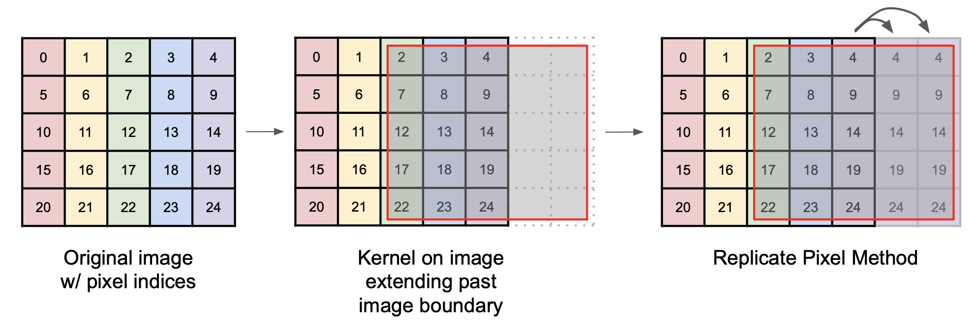
As promised earlier, we'll now discuss how to account for the case where the kernel extends beyond the boundary of the image, where pixel data is not defined. How can we obtain pixel "data" for, say, a pixel at
There are several ways to deal with this, and in filterutils.cpp, we have provided you some functions for this purpose:
getPixelRepeated()
// Repeats the pixel on the edge of the image such that A,B,C,D looks like ...A,A,A,B,C,D,D,D...
RGBA getPixelRepeated(std::vector<RGBA> &data, int width, int height, int x, int y) {
    int newX = (x < 0) ? 0 : std::min(x, width  - 1);
    int newY = (y < 0) ? 0 : std::min(y, height - 1);
    return data[width * newY + newX];
}
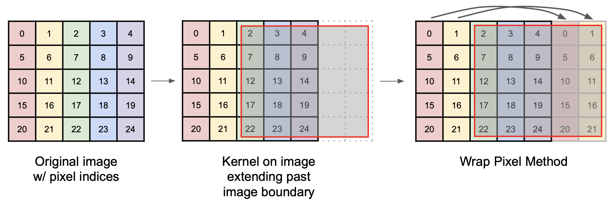
getPixelWrapped()
// Wraps the image such that A,B,C,D looks like ...C,D,A,B,C,D,A,B...
RGBA getPixelWrapped(std::vector<RGBA> &data, int width, int height, int x, int y) {
    int newX = (x < 0) ? x + width  : x % width;
    int newY = (y < 0) ? y + height : y % height;
    return data[width * newY + newX];
}
getPixelReflected()
// Flips the edge of the image such that A,B,C,D looks like ...C,B,A,B,C,D,C,B...
RGBA getPixelReflected(std::vector<RGBA> &data, int width, int height, int x, int y) {
    // Task 5: implement this function

    return RGBA{0, 0, 0, 255};
}
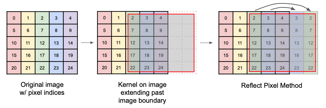
We have implemented functions (1) getPixelRepeated() and (2) getPixelWrapped() for you, and you are welcome to use either one of them in convolve2D().
Implement function (3) getPixelReflected(), and verify that it works.
Using Your Accumulated Values
Having accumulated your red, green, and blue values, you now need to update result with the new RGBA value.
Using redAcc, greenAcc, and blueAcc, update the result vector.
- You may find the
floatToUint8()utility function useful. - We only care about fully-opaque images, so you can set the alpha value to
.
Wrapping Up
Your result vector should now contain the output image's RGBA values. To display this image, we must overwrite the image data currently stored in data:
Copy the result vector into data. You may use a simple for loop, or std::copy (though this involves some knowledge of iterators).
Good work! You're done with the hardest part of this lab, and, in following sections, we'll use the convolve2D function you just implemented to perform some basic filtering. We will do so by defining different kernels for each filter, then convolving our input image with those kernels.
Identity Filter
An identity filter convolves the input image with an identity kernel, returning the original image.
In filterIdentity(), we have created an identity kernel for you. However, something is wrong with the kernel we created.
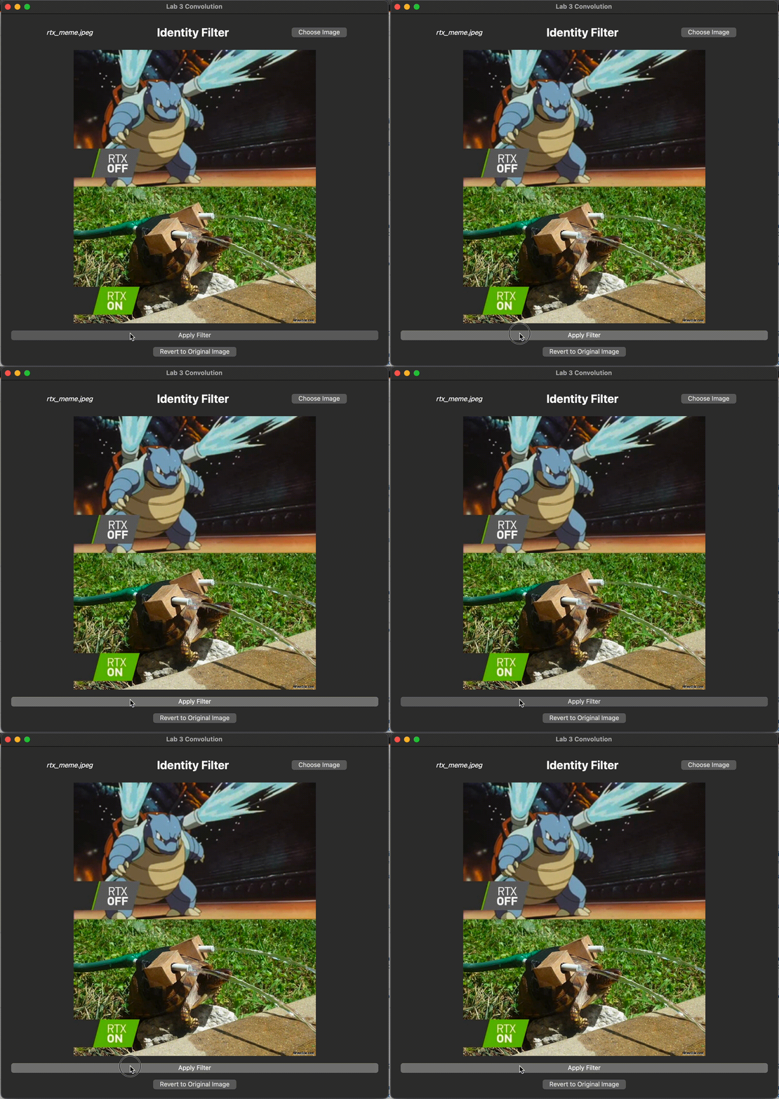
Run the program with identity as your command line argument. Convolution with the identity kernel should return the original image, but what is happening with our current identity kernel?
Identify the bug and fix it such that when convolving the image with identity kernel, it results in the original image. Be ready to discuss with the TA what the original bug was and how you fixed it.
Running and Testing:
Pass in identity as your command line argument.
Your (corrected) filter should produce the following output:
Shift Filter
A shift filter shifts the image by some number of pixels.
In filterShift(), initialize a kernel which, when convolved with an image, shifts the image one pixel to the left or to the right, depending on the value of shiftDir.
Optional task: implement createShiftKernel()
This function should create a shift kernel that is able to shift the image num pixels in the direction of shiftDir.
Call convolve2D(), passing in your kernel and appropriate canvas information. convolve2D() will convolve your image with the shift kernel.
Running and Testing:
Pass in either shiftLeft or shiftRight as your command line argument.
Your filter should produce the following output:
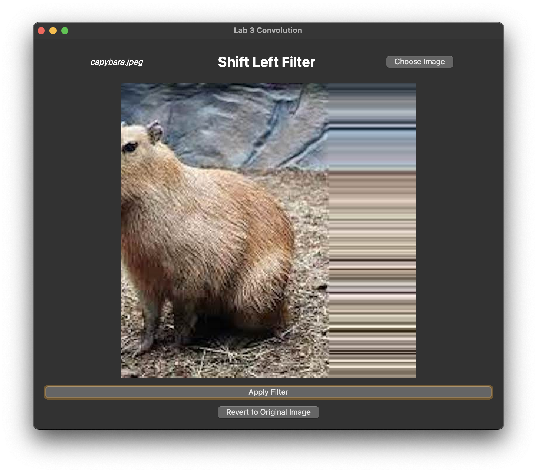
A left-shift filter applied many times to an image, using the getPixelRepeated() approach.
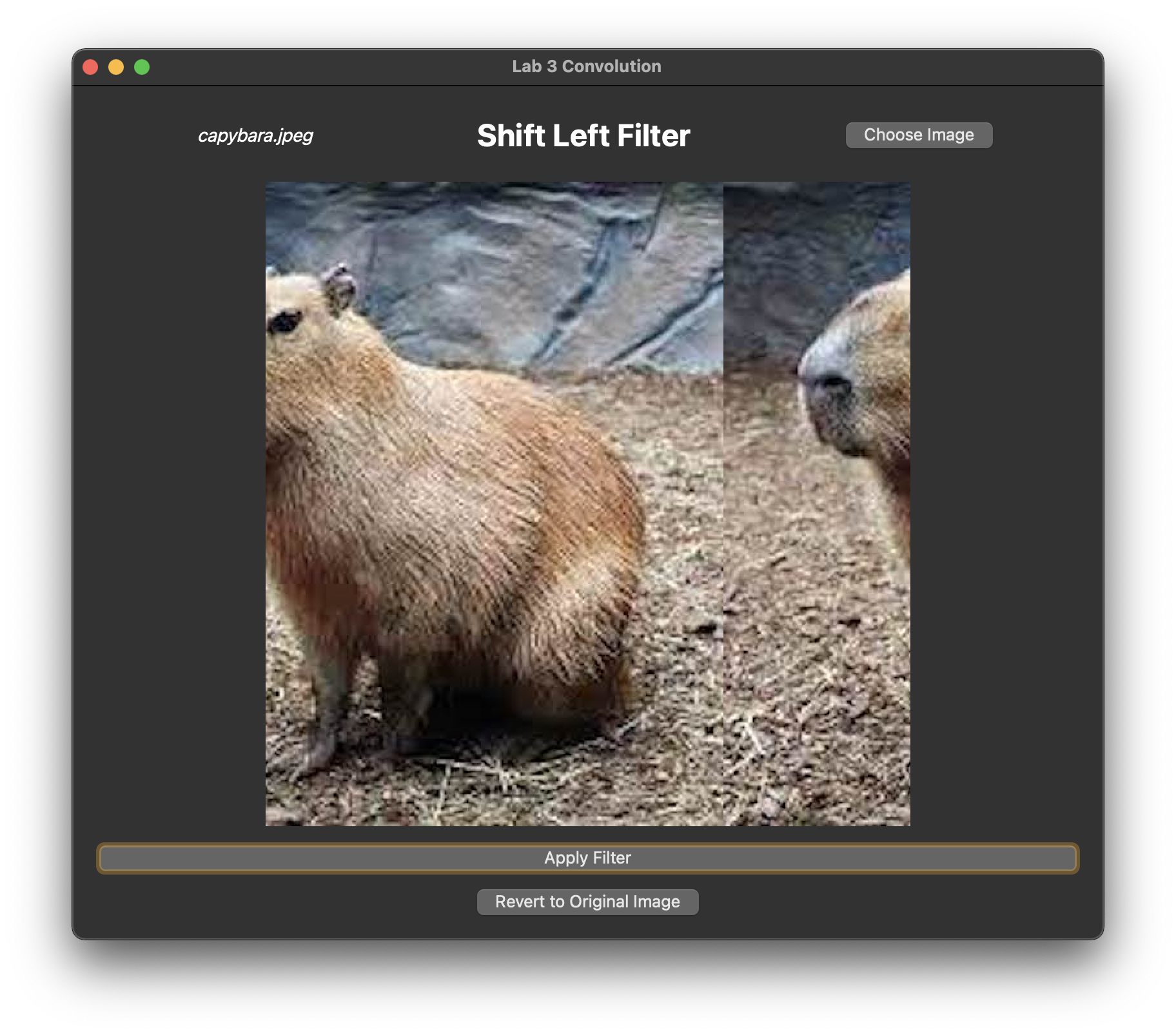
A left-shift filter applied many times to an image, using the getPixelWrapped() approach.
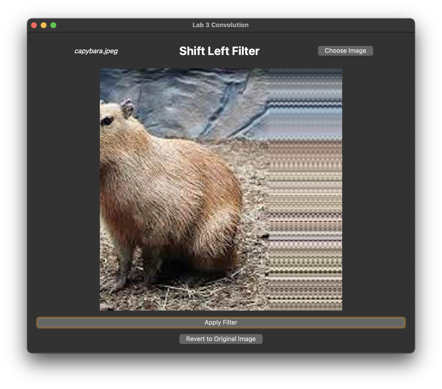
A left-shift filter applied many times to an image, using the getPixelReflected() approach. This one
shifts the image by 5px at a time.
Mipmapping
Now, let's move onto some practices with mipmapping to prepare you for Project 4: Antialias. As we have seen in class, bilinear filtering helps with antialiasing, but a fixed
Ideally, we would filter the texture with a filter whose size is proportional to the pixel's footprint on the texture. However, doing so would be prohibitively expensive at render time. Instead, we can precompute a series of downsampled versions of the texture, called mipmaps (short for "multum in parvo," Latin for "many things in a small place"). Each level of the mipmap is downsampled by a factor of
Downsampling
Generating mipmaps requires the ability to properly downsample an image. Thus, you'll need to implement a function that can take an image and scale it down by a factor, being sure to use a pre-filter to avoid introducing aliases. You will practice doing so with a box filter for this lab, and you should implement it as a separable filter for efficiency. Everything you need to know for this implementation has already been covered in great depth during the Sampling, Reconstruction, & Antialiasing lectures.
Important: This lab is meant to prepare you for Project 4: Antialias with some basic mipmapping functionality that you will extend in the project. In particular, here are some differences between what you are implementing in this lab for practice vs. what you are expected to implement in your project to receive full credit:
| This Lab | Project 4: Antialias | |
|---|---|---|
| Filter Type | separable box filter | separable triangle filter |
| Downsample Factor | fixed factor of | arbitrary factor |
| Next Image Generated From... | previous image | original image |
In horizontalBoxPass() and verticalBoxPass(), downsample the width and height by
Then, in downsampleBy2(), call the horizontalBoxPass() and verticalBoxPass().
Hint: How wide should each of the separated kernels be, and what are the weights?
Please refer to the lecture slides first to get a refresher on how to determine the width of your downsample kernel. Furthermore, because we are using a box filter, each weight is the same, and remember to normalize the sum of the weights across the kernel to avoid brightening or darkening the image. If some of the pixels in the kernel's current location are out-of-bounds, you should only normalize the weights accumulated across the in-bounds pixels to avoid brightening or darkening the image.
We know that this part could be a bit challenging, so we've provided some more detailed hints below to help you out, but we ask you to make a good-faith effort to figure out the answer on your own first before looking at the solution:
Solution: How do I find the width of the kernel?
As shown in the lecture slides, since we are downscaling, the radius of your downsample kernel should be
Expand for an example of normalizing by the correctly accumulated weights
Note: this example uses random kernel weights for illustration purposes and is not meant to be a correct downsample kernel.
Suppose your filter kernel has a width of 4 pixels with weights
On the contrary, if all pixels in the filter kernel's current location are in-bounds, you normalize the output RGBA value by dividing each channel by the sum of all the weights:
What do I do if the width or height of my input image is not a multiple of the downsample factor?
There are many ways to handle this, but for this lab and Project 4: Antialias, it is sufficient to round down the width and height of the output image to the nearest integer (i.e., discarding the extra row(s) or column(s) of pixels).
Mipmap Generation
Now that you have implemented downsampling, you can generate mipmaps of every level for every texture in your scene!
In generateMipmapChain(), create multiple mipmap levels by repeatedly calling downsampleBy2() on the previous level's image until the width or height of the image can no longer be halved (i.e., until the width or height is
In this lab, we will track your mipmaps in a std::vector<std::vector<RGBA>> data structure for visualization purposes, but in your project, think about the way you'll use these downscaled images in your raytracer, and choose an appropriate data structure to keep track of them.
What does the std::vector<std::vector<RGBA>> data structure store?
Each inner std::vector<RGBA> represents the pixels for the image (flattened into a 1D array) for a single mipmap level, and the outer std::vector<> is the list of all of those flattened mipmap level images.
Running and Testing:
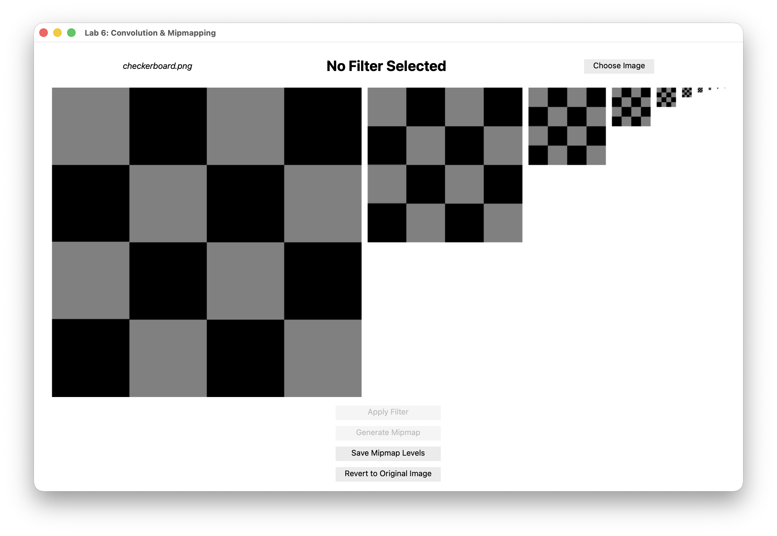
You are required to generate mipmaps with the checkerboard image provided in the resources directory. Be ready to show your output to your TA during checkoff!
-
checkerboard.png
Figure 13: Mipmap levels generated from checkerboard image -
Optional:
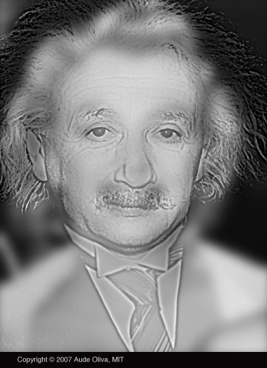
MonroeEinstein_AudeOlivia2007.jpgWhose face do you see in the mipmap levels? Try it out to find out!

Figure 14: Monroe Einstein
To confirm that your filter and downsampling work correctly, especially on the smaller mipmaps, you can save your mipmaps with the Save Mipmap Levels button in the application window. This will save all of your mipmaps to the mipmaps_generated/student_generations folder, and you can use an online pixel-by-pixel image comparison tool (like this one) to compare your mipmap levels with the provided reference mipmap levels in the mipmaps_generated/ground_truth folder.
You are more than welcome to use this to generate mipmaps for other images (whether from the resources directory, your own, or especially the Project 4: Antialias textures).
End
Congrats on finishing the Convolution & Mipmapping lab! Now, it's time to submit your code and get checked off by a TA. Be prepared to show the TA your working identity, shiftLeft, shiftRight filters and your generated mipmaps!
Submission
Submit your GitHub link and commit ID to the "Lab 6: Convolution & Mipmapping" assignment on Gradescope, then get checked off by a TA at hours.
Reference the GitHub + Gradescope Guide here.