Lab 7: Terrain
Please put your answers to written questions in this lab, if any, in a Markdown file named README.md in your lab repo.
- Please note that, for the entirety of this lab, we will be using the
z-up convention. That is,glm::vec3(0, 0, 1)points vertically upwards. - Also remember to set your working directory!
- This lab won't have content directly related to upcoming projects, but it is important content that you could keep in mind as a component of the final project!
Introduction
Hello, and welcome to the Terrain lab!
In lab 5, we used 2D arrays containing intersection information to calculate lighting. In this lab, we will instead use 2D arrays containing height information to construct geometry.
First, we'll implement a noise function which we can use to generate height maps; then, we'll experiment with ways to add detail and color to our scene. Let's get started!
Objectives
- Learn about the basics of procedural noise,
- Understand how scaling and adding noise creates interesting detail, and
- Gain familiarity with non-implicit geometry and per-vertex data.
Procedural Noise
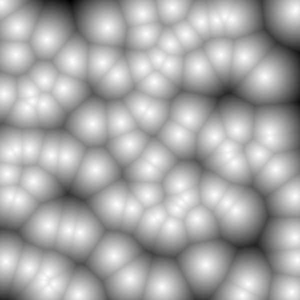
Procedural noise is used in graphics to create randomized data with certain desirable properties (e.g. continuity). It is used to make a wide variety of assets, including geometry and textures.
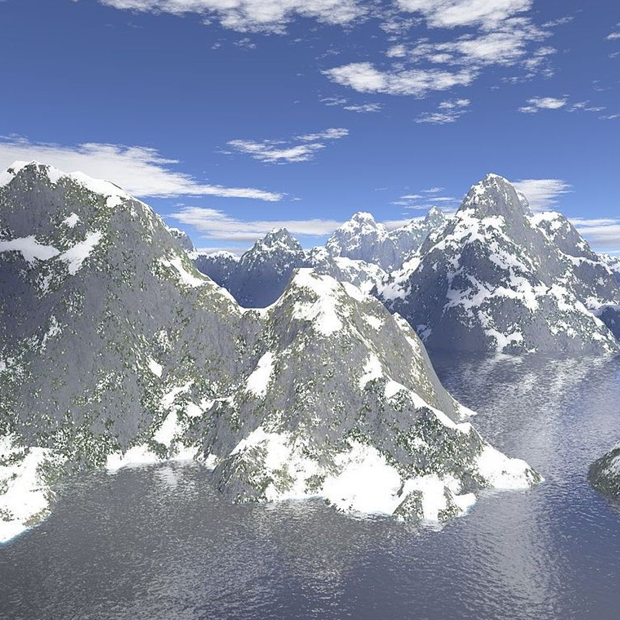
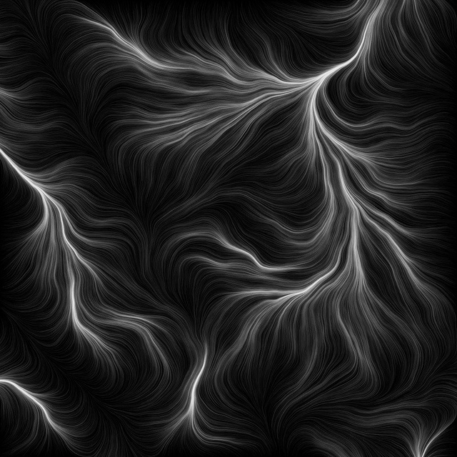
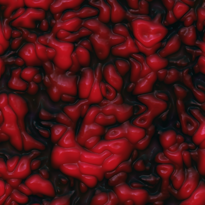
As you can see from these examples, well constructed noise can be used to create incredible scenes and images from complete (pseudo-)randomness!
In this lab, we will attempt to use procedural methods to generate 2D textures, which we'll use as height maps from which we can construct geometry. Before we can get into that, though, we must choose a noise function:
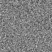
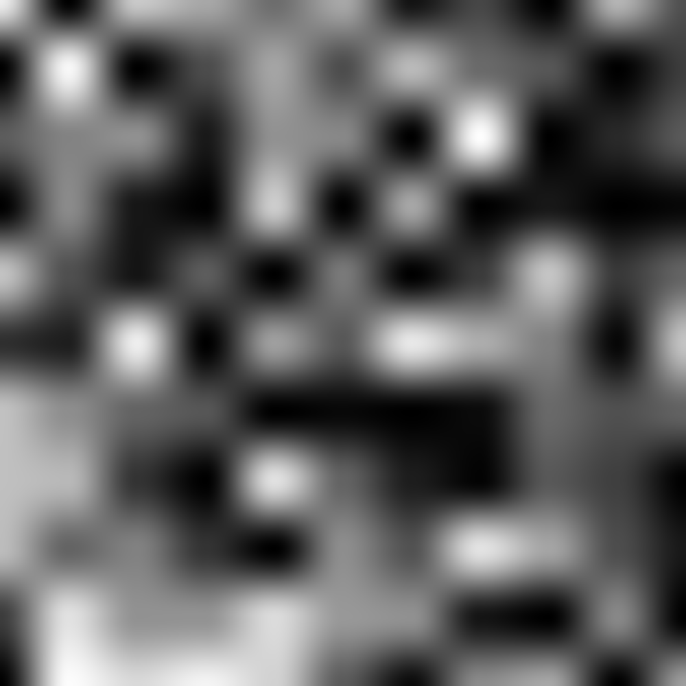
White Noise
White noise is one of the simplest forms of noise. Every pixel is assigned a random value, independent of the values of its neighbors.
- Pros:
- Easy to implement
- Very fast
- Cons:
- "Too noisy" for certain use cases
- Discontinuous
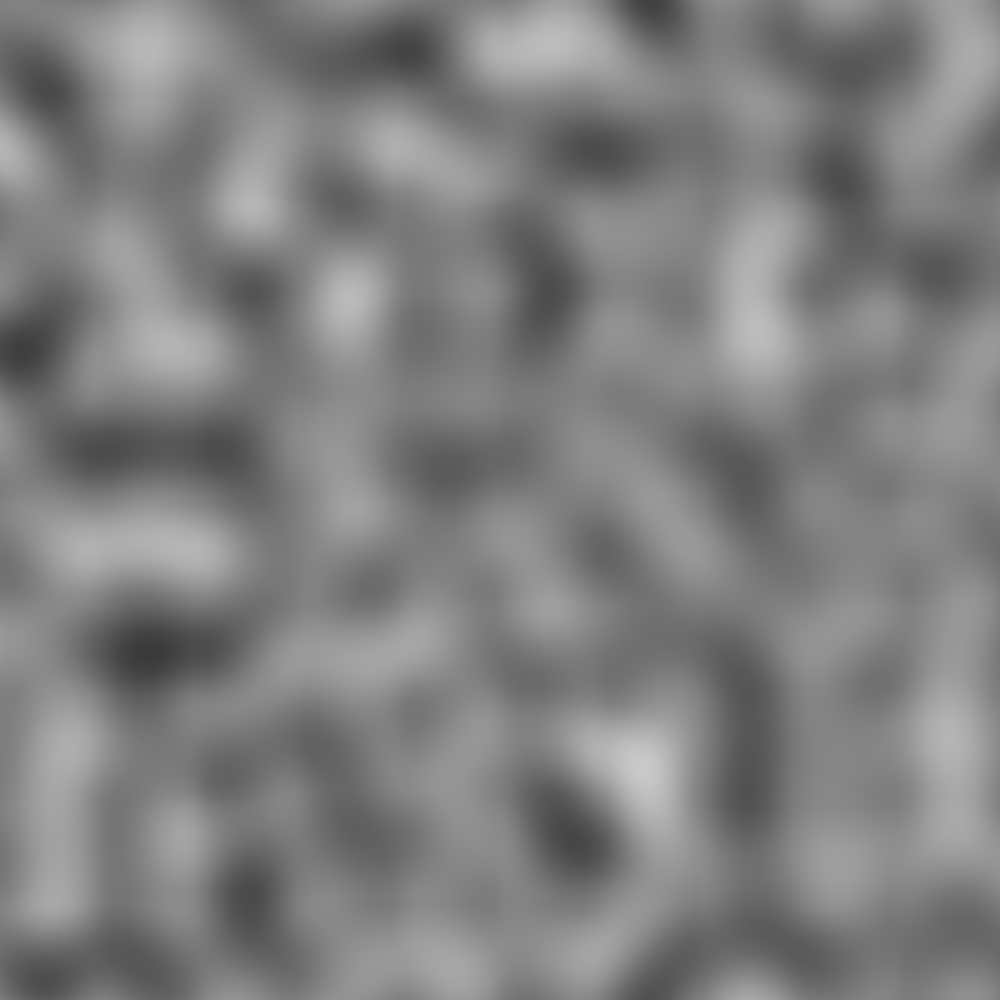
Value Noise
The next simplest form of noise is value noise. Value noise is essentially white noise run through a scaling filter: a grid of white noise values is first generated at lower resolution, then scaled up.
Equivalently, value noise is simply bilinearly-interpolated white noise.
- Pros:
- Fairly easy to implement
- Pretty fast
- Locally continous
- Cons:
- Resulting noise is visibly aligned to the pixel grid
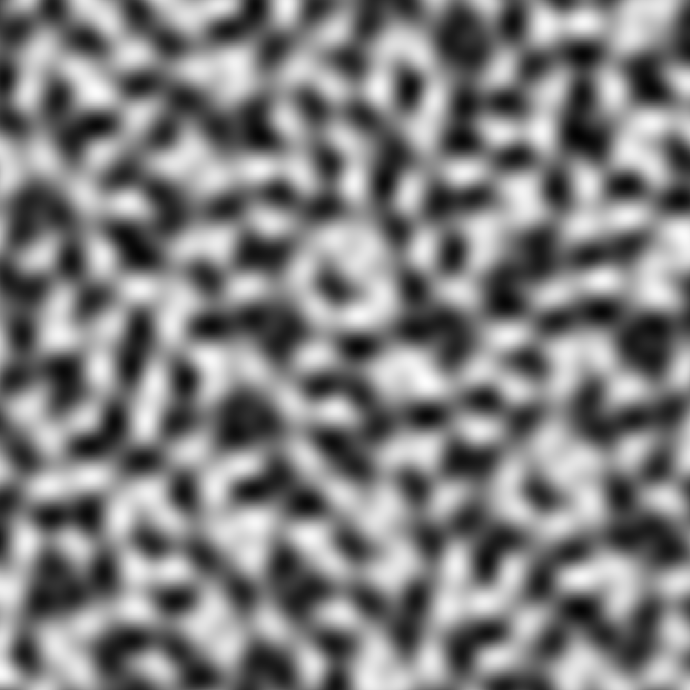
Perlin Noise
Next, we have Perlin noise, which is what you'll be implementing in this lab. You can think of Perlin noise intensity as being some function of a grid of vectors, instead of a grid of values like in value noise.
- Pros:
- Locally continuous
- Resulting noise looks more organic, and is less visibly aligned to the pixel grid
- Cons:
- More challenging to implement
- Can be very inefficient if implemented poorly
While Perlin noise is (very) widely used, it has flaws beyond those which we listed above. Its creator, Ken Perlin, has himself designed an alternative to Perlin noise, known as Simplex noise. Read more about it here!
Generating Perlin Noise
Now that we've taken a brief tour of the types of procedural noise available to us, we can dive into actually generating some of our own.
In this section, you'll learn how you can compute the intensity of Perlin noise at some point in 2D space, and implement a function (computePerlin()) to do exactly that. This will enable us to create (if we wanted to) an image like Figure 5. Here's how it works:
Before all else, we prepare an infinite, integer-indexed grid of random direction vectors.
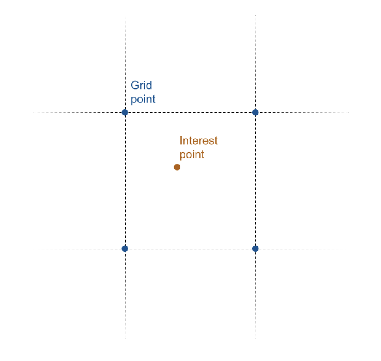
- Given an interest point, we can find the four grid points closest to that point.
- Then, we can obtain the four offset vectors pointing from each closest grid point to the interest point.
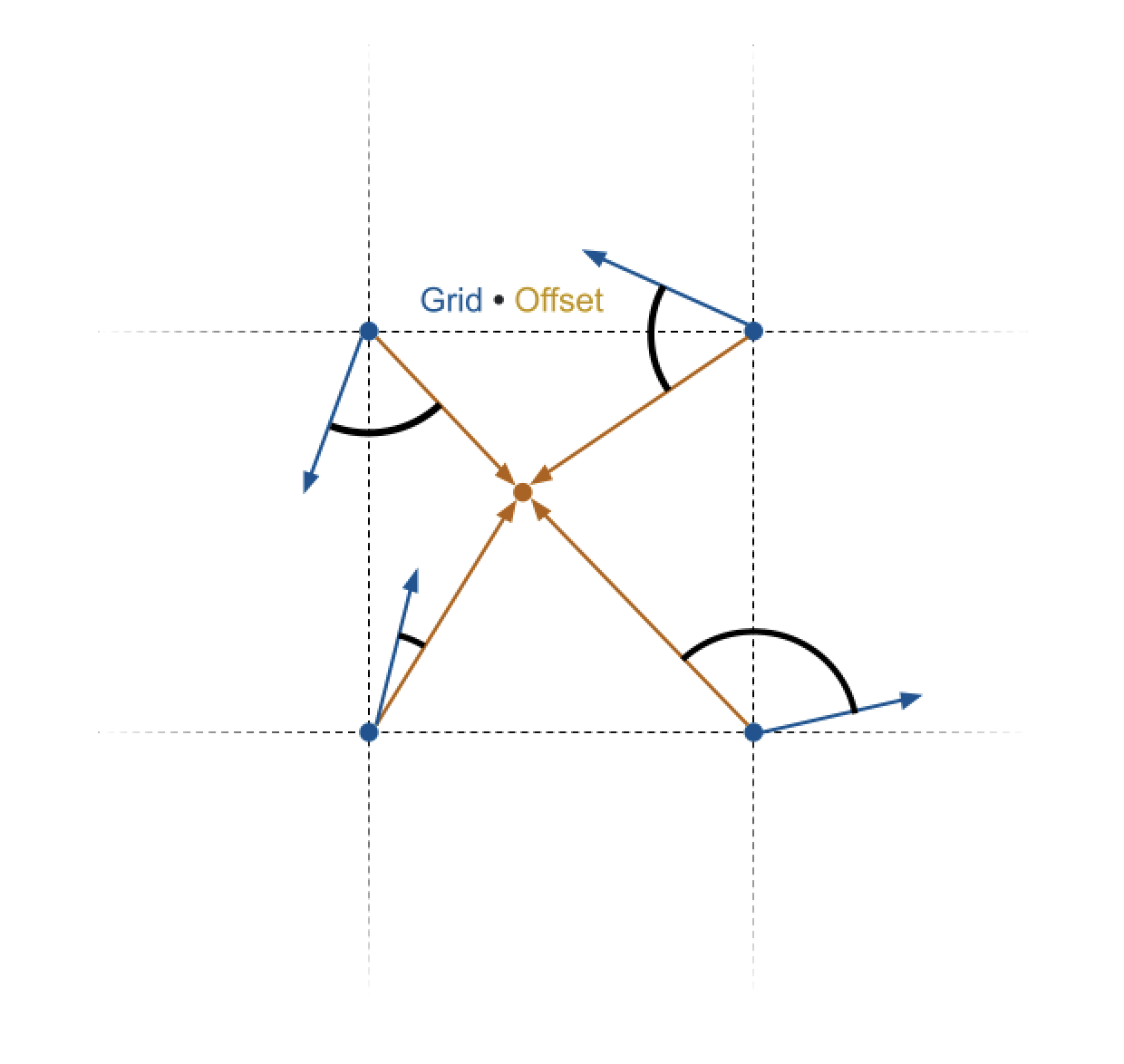
- Next, we can compute the four dot products between these grid points' offset vectors and their random direction vectors.
- Finally, we use an interpolation function to combine the four dot products into a single intensity value.
Now, to produce something like an image, we can then repeat steps 1-4 for each interest point (i.e. pixel), and obtain an intensity value for each.
Don't worry, we'll walk through this step-by-step. To get started, please open terraingenerator.cpp and locate the computePerlin() function, which is where most of our work will be done.
Random Direction Vectors
Before all else, we prepare an infinite, integer-indexed grid of random direction vectors.
Instead of actually storing an explicit grid, which would be very inefficient, we instead provide a function, sampleRandomVector(). This returns the random direction vector "stored" at a particular coordinate; it is both coherent (the same input row and column produces the same output vector) and infinite in extent, so it acts as an infinite grid.
Please take a look at sampleRandomVector(), and understand how to use it.
Getting The Four Closest Grid Indices
- Given an interest point, we can find the four grid points closest to that point.
Remember that computePerlin() takes in floating point coordinates from the real plane,
Thus, given some point of interest in the form of the input floating point coordinates, we must first obtain the integer indices of the four closest grid points. The simplest way of doing this is rounding our floats down to the nearest integer, then adding 1 to get the adjacent indices.
Within TerrainGenerator::computePerlin(), obtain the integer coordinates of the four closest grid points.
You don't have to store these explicitly if you don't want to.
Computing The Offset Vectors
- Then, we can obtain the four offset vectors pointing from each closest grid point to the interest point.
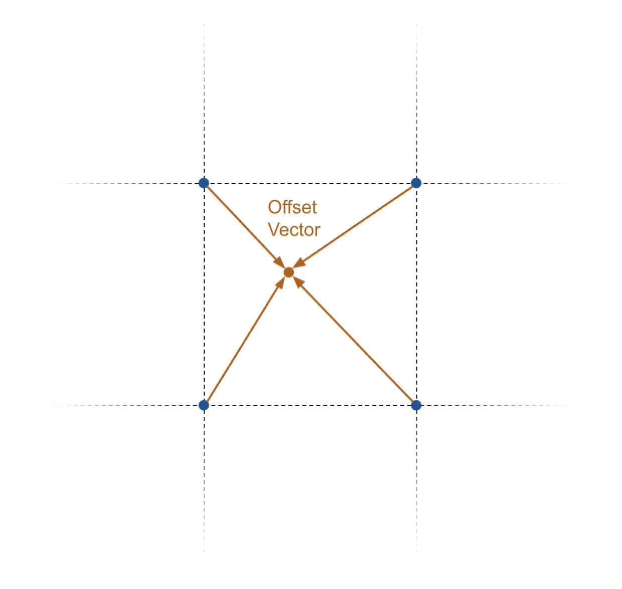
Using the coordinates of the four closest grid points and the input location, compute the four offset vectors from the grid points to the interest point. Do NOT normalize these.
Computing Dot Products
- Next, we can compute the four dot products between these grid points' offset vectors and their random direction vectors.
In your code, uncomment the following lines:
// Task 3: compute the dot product between the grid point direction vectors and its offset vectors
float A = ... // dot product between top-left direction and its offset
float B = ... // dot product between top-right direction and its offset
float C = ... // dot product between bottom-right direction and its offset
float D = ... // dot product between bottom-left direction and its offset
Compute four dot products, one for each grid point's pair of offset vectors and direction vectors, and assign the values to the corresponding float A, float B, float C, and float D variables. This will yield four floating point values.
float Arefers to the dot product for the top-left grid pointfloat Brefers to the dot product for the top-right grid pointfloat Crefers to the dot product for the bottom-right grid pointfloat Drefers to the dot product for the bottom-left grid point
Interpolating The Dot Products
- Finally, we use an interpolation function to combine the four dot products into a single intensity value.
Our next step is to interpolate these four dot products to produce a final intensity value for the point of interest. How do we do that?
Interpolation
You may not be aware of this, but you've actually already implemented interpolation—you did that when blending brush and canvas colors in Brush, and when averaging pixels when scaling in Filter.
Interpolation is simply the "mixing" of two values to produce a new one, based on an input "mixing" parameter.
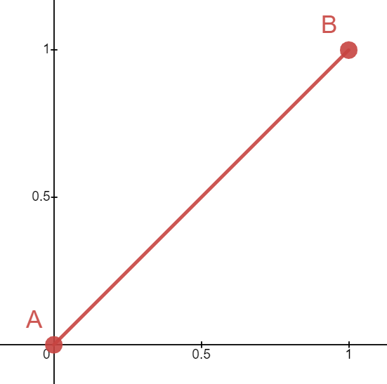
The simplest method, linear interpolation, takes the form below. This should look very familiar!
Here,
Observe that when
Skipping ahead a little, if we were to use we use linear interpolation to combine the dot products for our terrain generator, we'd get the following result:
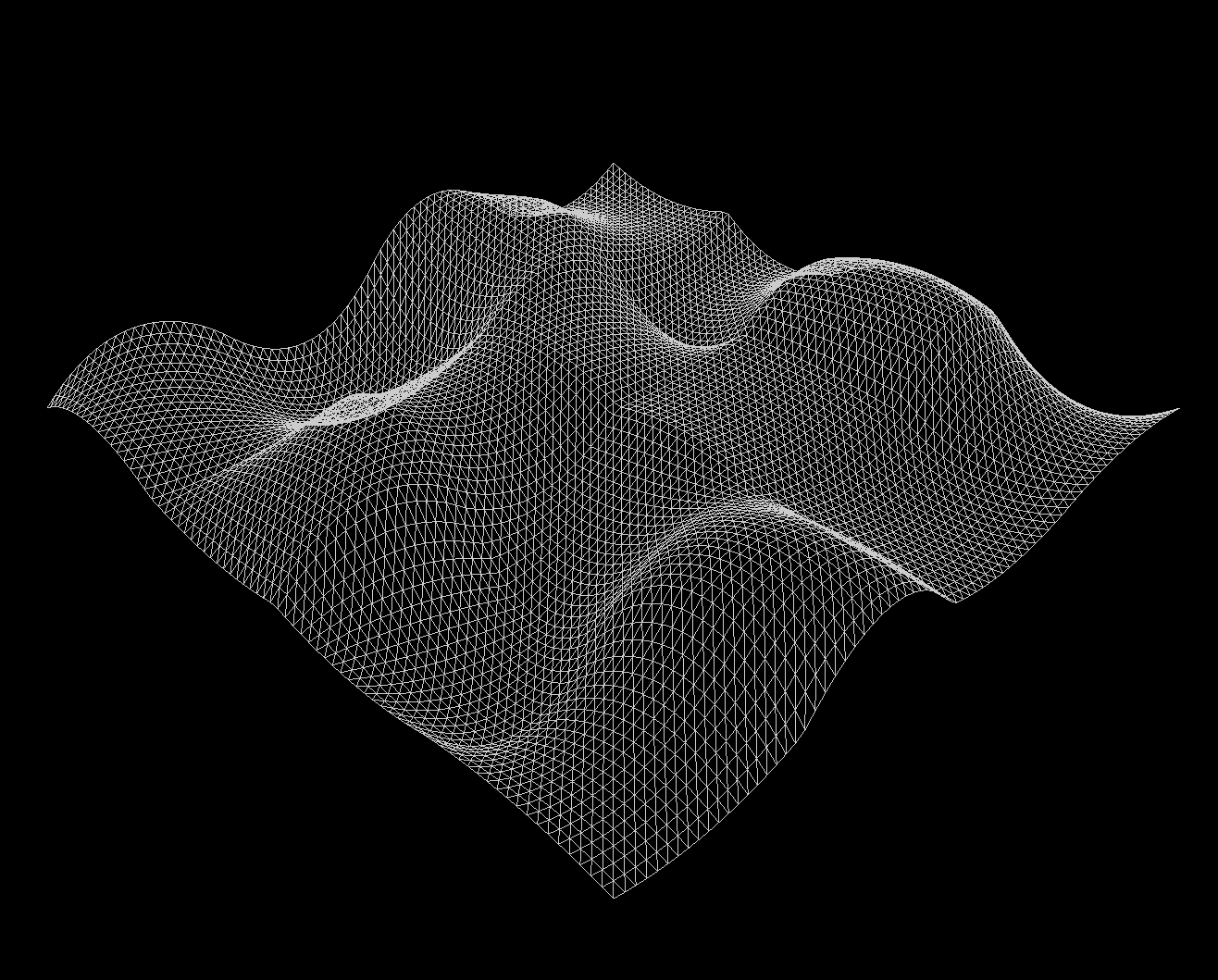
Notice that the linear interpolation function leaves the surface way too angular for "realistic" terrain. Ideally, we'd like to be able to smooth out those curves. This is where easing functions come in!
Easing Functions
An easing function (also known as a shaping function) has the following properties:
We can use an easing function to re-map our linear slope to whatever curve we'd like. To do this, we can use apply it on our mixing parameter
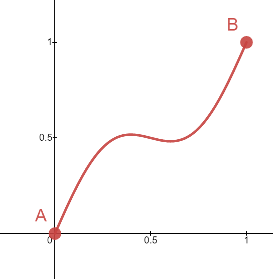
The choice of easing function is a creative design decision. For example, you could choose a weird, curvy function if you really wanted to produce something like this:
Since we'd like to generate reasonable-looking terrain, we recommend using a cubic easing function, given by the formula
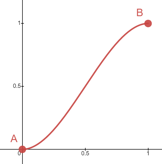
Implement the helper function, interpolate(). Follow the equation given above, and use any easing function you like—we recommend the cubic one, but there are many to choose from!
Extra: additional resources about easing functions
This website provides a cheat-sheet of common easing functions used in website styling (CSS), but it can give you a general sense of the types of things easing functions can do.
For more information about easing functions as they pertain to generative art and shaders (lab 10), The Book Of Shaders has an entire chapter devoted to them.
Bilinear Interpolation
Now, let's return to our attempt at generating Perlin noise, where we left off at trying to combine four float values into one noise intensity value. This is where we put our interpolation function to work. We have a problem, though: we defined our interpolation to work based on two values and one mixing parameter, so how are we going to combine four values?
The solution is to perform multiple interpolations, then compose them to get one final value.
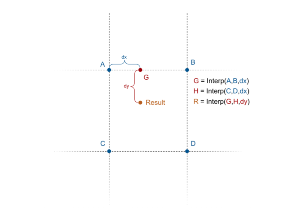
In the image above, we have values
- get
by interpolating between and - get
by interpolating between and , and, finally - get
by interpolating between and
When linear interpolation is used with this strategy, the resulting algorithm is known as bilinear interpolation. This strategy can be extended to higher dimensions, too (e.g. trilinear interpolation in 3D), though you won't need to do that in this lab.
Now that has all been covered, us TA's have tried to complete the implementation of the computePerlin() function by writing this four-way interpolation, but it doesn't look right and we need your help!
Back in computePerlin(), uncomment the following line:
// Task 5: Debug this line to properly use your interpolation function to produce the correct value
return interpolate(interpolate(A, B, 0.5), interpolate(D, C, 0.5), 0.5);
Here, the TA's have tried calling your interpolation function to merge the four dot product results into a single height value. But when we run the code, it doesn't look like the expected result:
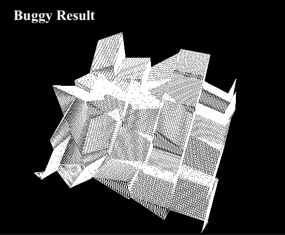
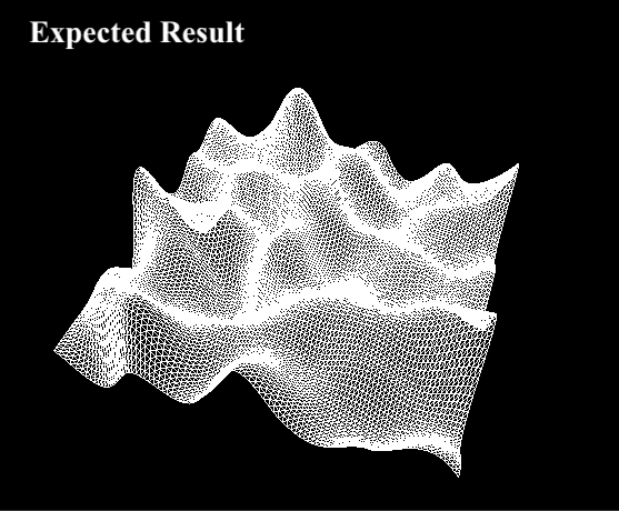
- Using the what you learned about bilinear interpolation, fix the
interpolate()call(s) so that the terrain looks similar to the expected result. - Be prepared to briefly explain what the bug is and how you fixed it.
Note: Since Perlin noise uses random direction vectors, your output might not exactly match the expected output. This is fine, as long as you see a smoother terrain similar to the expected one.
Introducing Octaves
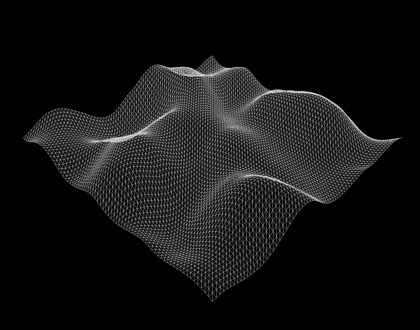
We can generate basic, bumpy terrain. Great! However, it still looks somewhat unnatural, and a little too smooth, so let's attempt to make our terrain more rugged. To do this, we'll add multiple octaves of noise, at different scales!
Modifying Our Perlin Noise
The first thing to understand is how to modify Perlin noise in the first place. We have two main ways we can do this: scale its amplitude, or scale its frequency.
Take a look at getHeight(), where we call computePerlin():
-
By scaling the output of
computePerlin()(i.e. multiplying by a constant), we can produce noise at higher or lower amplitudes. -
By scaling the inputs of
computePerlin(), we can produce noise at highter or lower frequencies.
Within getHeight(), scale the output of computePerlin() to generate noise with a different amplitude. What happens? This should be fairly straightforward to understand.
Next, scale the inputs to computePerlin() to generate noise with a different frequency.
What do you see when you multiply the inputs by a larger / smaller number? Can you explain why this happens? Write this down for your checkoff!
Combining Octaves
Now that we know how to modify our noise, how can we select different amplitudes and frequencies of noise to combine?
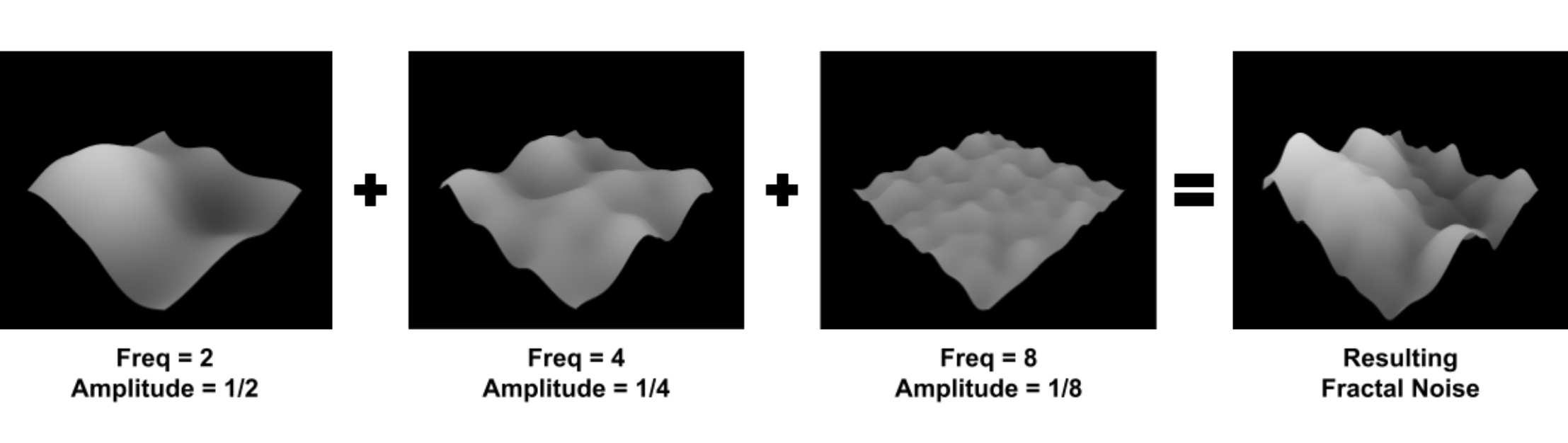
One technique which gives natural-looking results is to combine noise with frequencies that are scaled by by powers of two. Doubling the frequency gives us the next "octave" of noise (a term borrowed from music).
But, we have to be careful when doing this. If we naïvely added different frequencies of noise, the higher-frequency noise would completely overpower the lower-frequency noise. To avoid this, whenever we double the frequency of the noise, we typically also halve its amplitude.
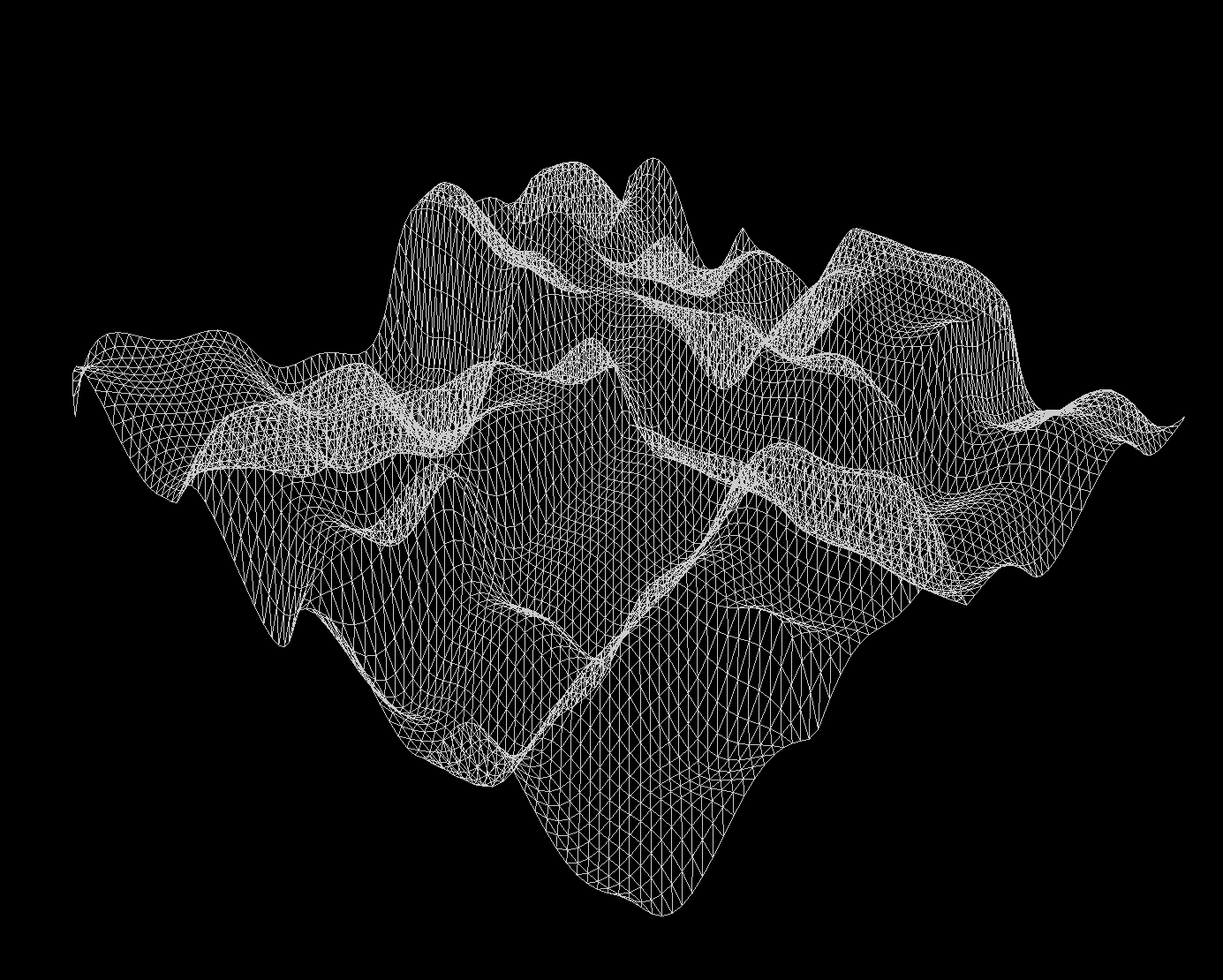
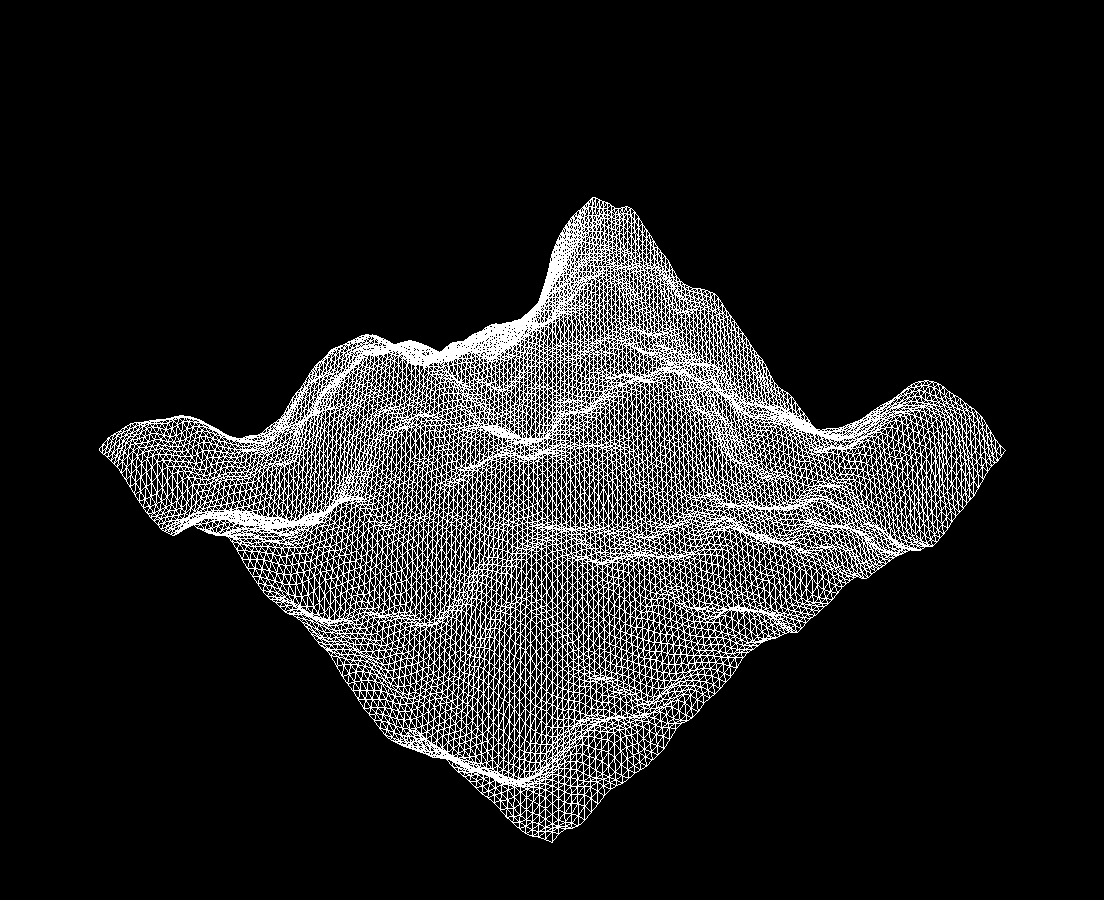
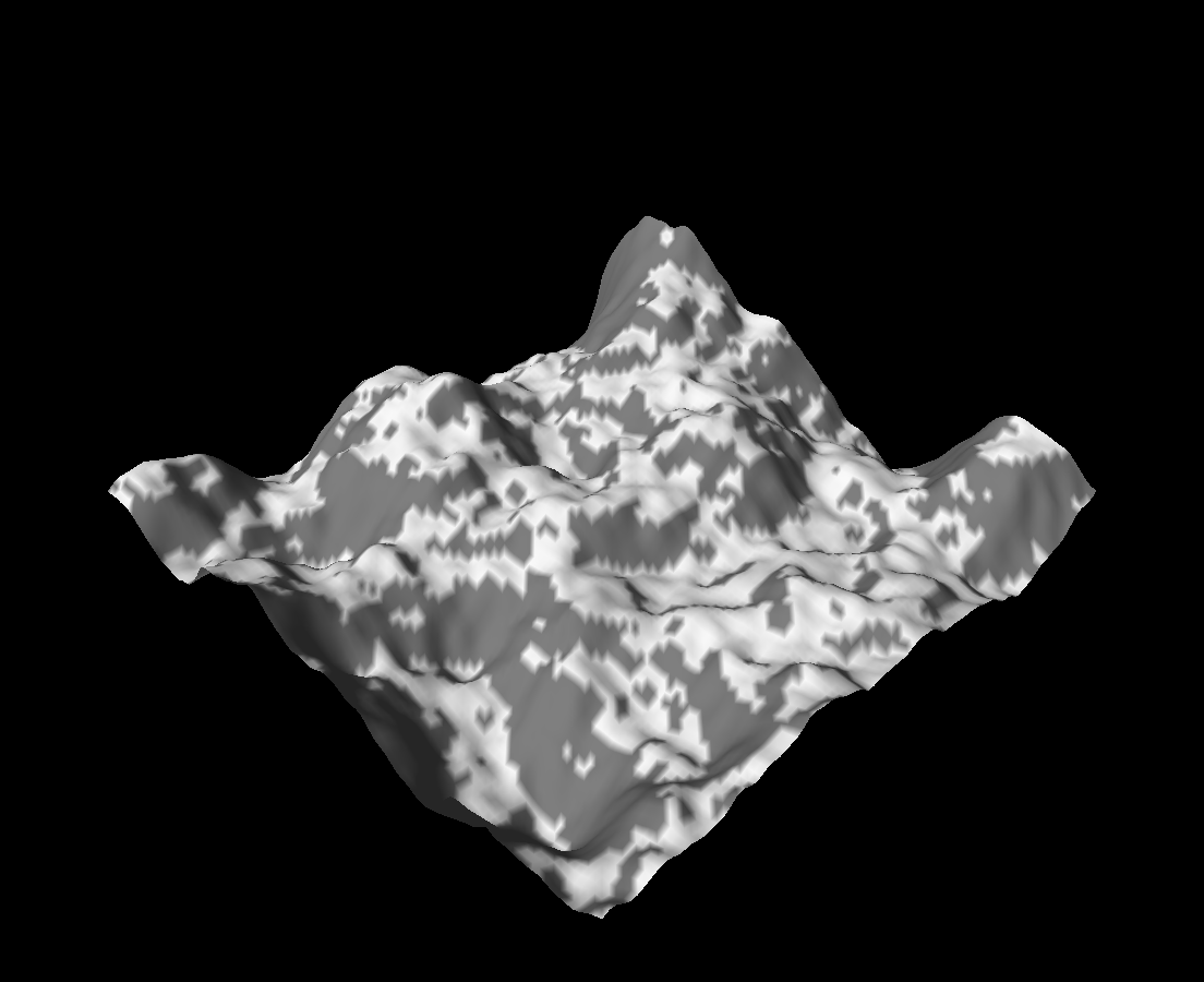
In getHeight(), call computePerlin() multiple times. Add at least four different noise octaves together, each with whatever amplitude and frequency you like, to generate rugged terrain.
Once you finish, you should now see something like the image below (the one from earlier):
Normals & Colors
At this point, you've used Perlin noise as a height function, to create rugged, mountainous terrain. However, there isn't really any variation in color or shading, so the scene looks kind of bland.
To fix this, we'll implement per-vertex normals to enable lighting effects, and introduce a per-vertex color based on the height and slope of the surrounding terrain. The end goal will be gray, stone-like mountains with white "snow"-covered peaks!
To start, switch m_wireshade to false in the constructor.
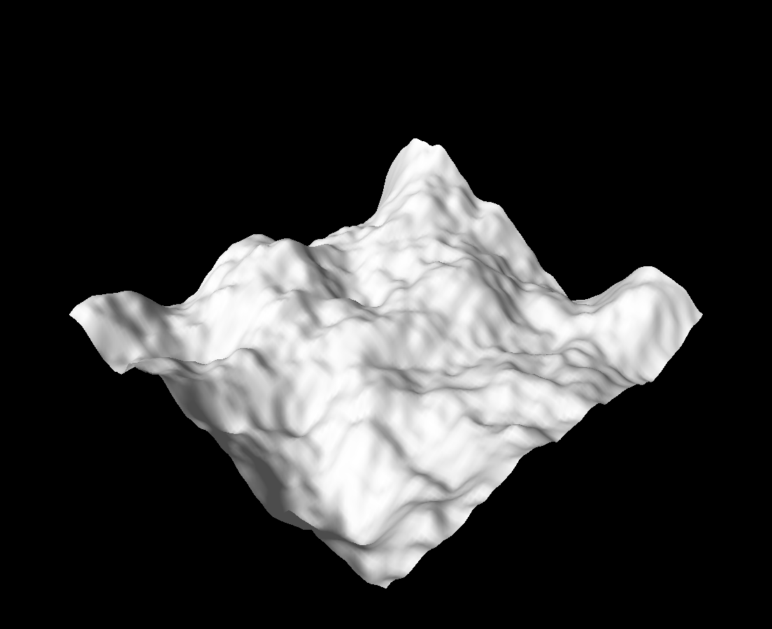
Your terrain should now appear as a solid white-gray color.
This is because the vertex colors are set to white in getColor(), the vertex normals are set to point straight up in getNormal(), and there is some basic lighting due to a directional light shining on the scene from the left—but it's all wrong because of the normals!
Getting The Normal
We are now faced with the problem of computing the correct normal for any given vertex. As the geometry is procedurally generated, we cannot use the same analytic approach as we did for implicit geometry. Instead, we need an algorithm for computing the normals given arbitary geometry.
First, we consider a vertex
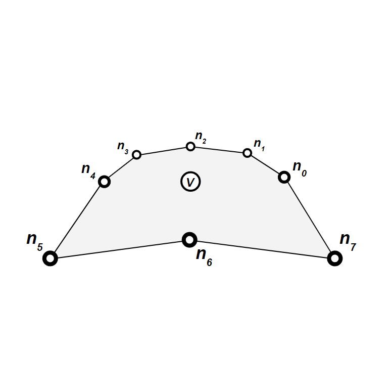
We can then group the vertices into 8 triangles, such that all triangles have
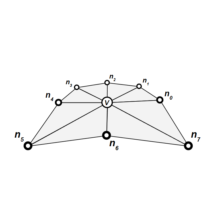
To compute the normal for such a triangle, we must first find its vertices' positions using something like getPosition(). We can then take the cross product
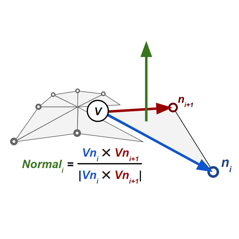
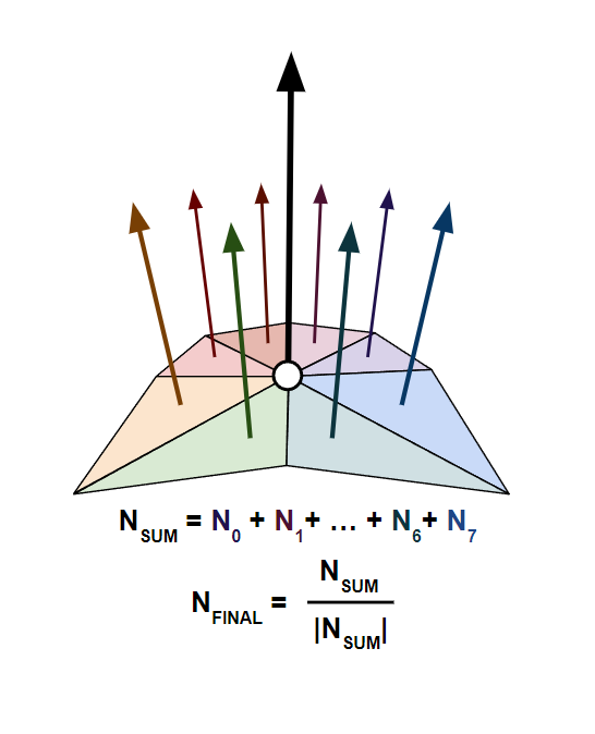
This gives us 8 normals, which we can average (equivalently: sum then normalize) to find the final normal for
Up to this point, we've neglected boundary cases. However, are there actually any boundary cases in our problem?
Despite what the comments describing getPosition() say, there's nothing actually stopping us from getting the position of a vertex outside of our plane. In fact, since we've defined an infinite grid of random vectors, and we've defined a computePerlin() function that works anywhere, getPosition() will work as expected for any integer coordinates!
Thus, we don't have to account for any boundary cases, and can assume that every vertex has 8 neighbors, as usual.
In the getNormal() function, implement the above algorithm for computing the normal of the specified vertex. You should now see something like the image below:
Extra: I need help!
This is the most challenging task of this lab, but that's not really saying anything.. you just have to iterate over some cleverly-ordered neighbor indices and accumulate normals.
That said, we know Intersect is really rough going, so we've provided the implementation here if you'd like to skip this task. Please at least attempt it first, though!
Setting The Color
Our goal is to make this terrain look like gray, stone-like mountains with white "snow"-covered peaks, but right now everything is plain white. So, our next task is to define some per-vertex color (actually, grayscale intensity) for each point.
There are many ways to do this, but for this lab, we'll explore just two basic techniques. Feel free to experiment with them however you like, or go beyond, and implement your own coloring heuristics.
By the way, remember that we're using the z-up convention in this lab, so glm::vec3(0, 0, 1) points vertically upwards!
Extra: y-up and z-up conventions
As we mentioned earlier, we're using z as the up vector in this lab. This runs contrary to our use of y as the up vector in the other CS 1230 assignments you've seen so far.
We can say that Lab 7: Terrain uses the z-up convention, whereas Project 3: Intersect uses the y-up convention.
The issue of y-up vs z-up conventions extends into commercial computer graphics software: both Maya and Unity use y as the up vector, but Blender and Unreal Engine use z as the up vector.
In different contexts, you might end up using different conventions—you might one day have to convert between them, too!
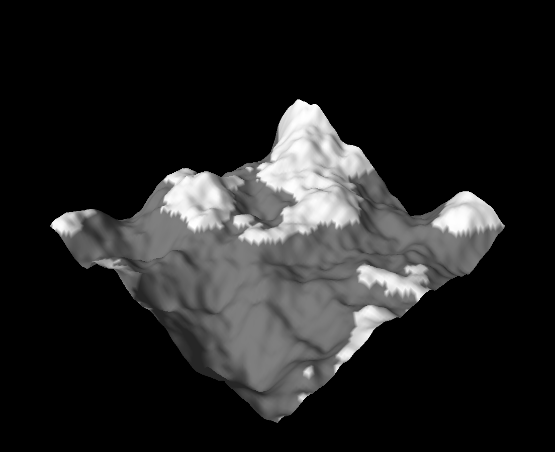
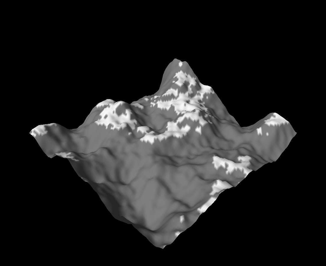
Implement getColor(). Try at least these three approaches:
- Set the color to white if the vertex is above some height (
zvalue), and gray otherwise. - Set the color to white if the vertex normal is "close to" vertical, and gray otherwise. How can you use dot products to achieve this?
- Combine both (1) and (2).
You should now see results like the ones below. Frankly, these overly-simple implementations of getColor() result in rather ugly outputs, but they're at least a start!
Optional Task: Easing The Color
The nature of computer graphics and generative art is that lots of it is highly qualitative; but we can probably agree that our getColor() function can be improved. The harsh boundary between white and gray regions is especially weird. How can we fix this with what we've learne so far?
Optional Task:
Earlier, you learned to use easing functions to map a [0,1] range to a more interesting shape (i.e. not a straight line).
- A vertex's
zposition varies from some minimum, to some maximum height based on your summed up amplitudes. - The dot product of its normal with the up vector also varies between
[-1,1].
Can you come up with a better approach, perhaps involving easing functions and the above data, to get a vertex's color?
End
Congrats on finishing the Terrain lab! Now, it's time to submit your code and get checked off by a TA.
Submission
Submit your GitHub link and commit ID to the "Lab 7: Terrain" assignment on Gradescope, then get checked off by a TA at hours.
Reference the GitHub + Gradescope Guide here.