Project 2: Filter (Algo)
You can find the handout for this project here. Please read the handout before working on this algo assignment!
Convolution
Discrete Convolution
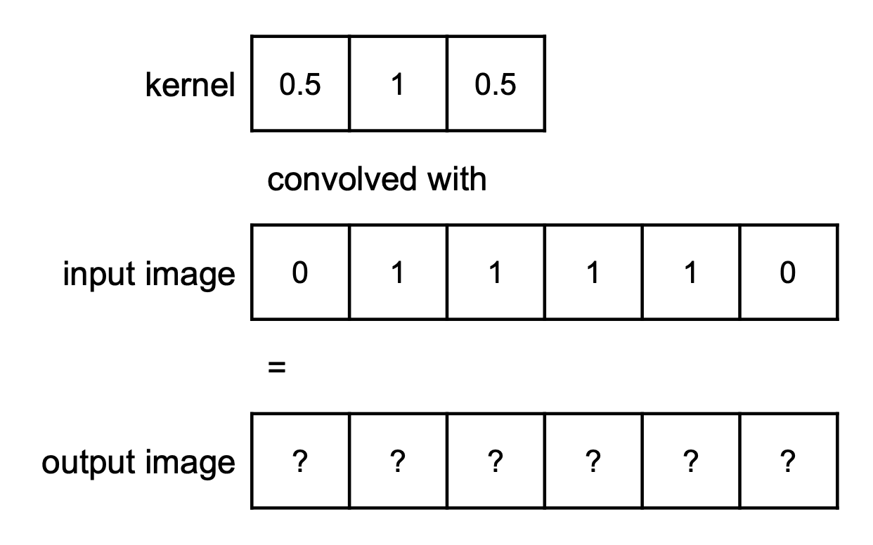
You are given the following 1D kernel and input image. Assume that any pixel outside the bounds of the input image has value 0 (i.e. the image is zero-padded).
What is the output image when the kernel and image are convolved with each other? Present your answer as a vector of size 6, representing the output image.
Continuous Convolution
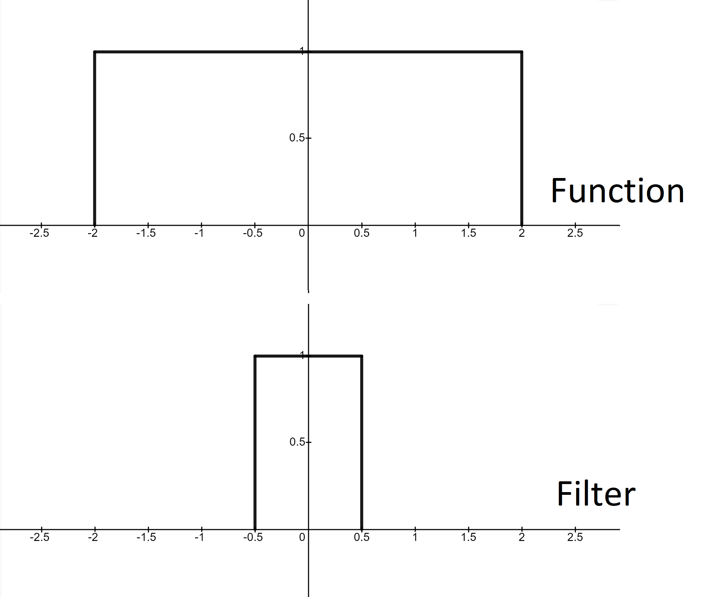
Convolve the below function and filter. What is the value of
Visualizing Convolution
Draw the shape of the output function obtained in the previous question (figure 2).
Blurring
Let's try to generalize our solution to the earlier discrete convolution problem.
Consider a 1D kernel
All of
, , and can be considered as 1D arrays storing intensities where gives the intensity of the -th pixel. Remember that the kernel is zero-indexed so gives the left-most value in the kernel array.
We are interested in writing out this convolution as summation over the values of
You may ignore edge effects for the purposes of this question (i.e. feel free to "incorrectly" index out-of-bounds).
Scaling
Scaling Up
What is the filter support width when you scale by a factor of
Scaling Down
What is the filter support width when you scale by a factor of
Naïve Back-mapping
Recall that back-mapping refers to finding the correct filter placement given a pixel in the output image.
The naïve back-map function is
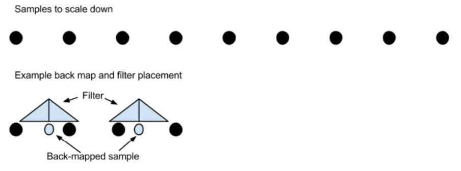
Suppose we wanted to scale down a 9-pixel 1D image by a factor of
Draw a picture to show where we would sample the original image using the naïve back-map function. Please include an illustration of the filter above each sample point.
Correct Back-map
Draw another picture to show where we would sample the original image using the correct back-map function. Again, please include an illustration of the filter above each sample point.
Duality of Domains
Visualizing Sinc and Box Duals
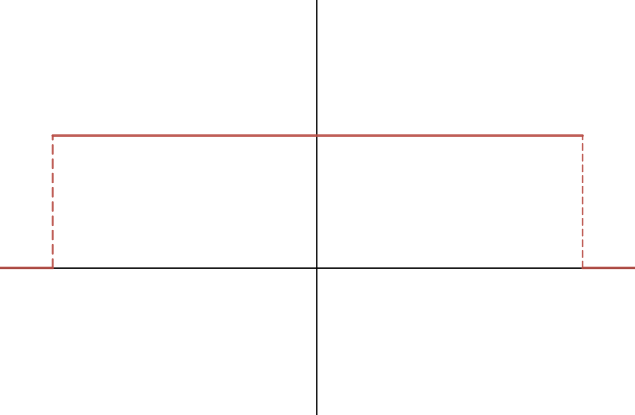
Take a look at the box function in figure 4 (left) below. Its dual in the frequency domain is the sinc function, in figure 4 (right). Note that there are no labels on the axes, by design.
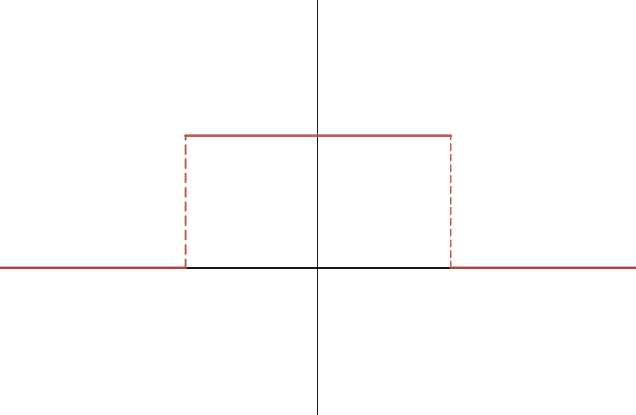
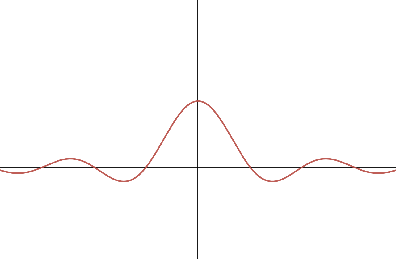
Please sketch the dual of the box function in figure 5. Your drawing doesn't need to be perfectly accurate; we just need to see that you get the idea.
Approximating Sinc
What do we usually use to approximate the sinc function, and why do we have to make this approximation when translating these theoretical concepts into code?
Sampling in the Frequency Domain
If we're sampling a continuous function at a frequency of
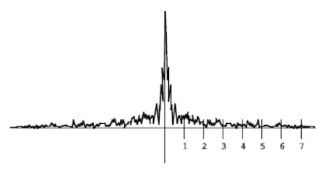
Frequency Plots
Now, examine the following frequency plot of a 1D, continuous signal. If you were going to sample this signal at a rate of 8 samples per unit, to avoid aliasing, you would use what we know about the Nyquist limit to pre-filter it. Sketch the new frequency plot after someone has performed this pre-filtering step optimally.
Submission
Submit your answers to these questions to the "Project 2: Filter (Algo)" assignment on Gradescope.