Project 2: Filter (Algo Answers)

You can find the handout for this project here. Please skim the handout before your Algo Section!

You may look through the questions below before your section, but we will work through each question together, so make sure to attend section and participate to get full credit!

Convolution

Discrete Convolution

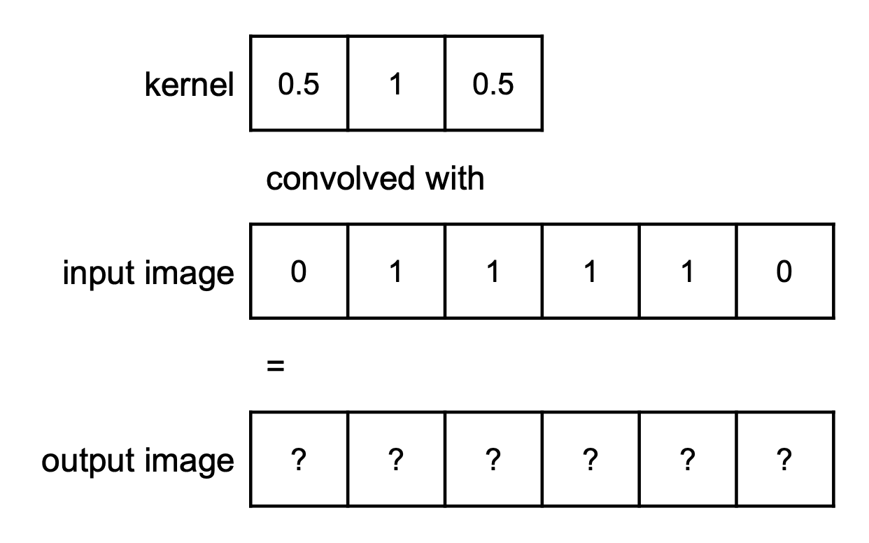
You are given the following 1D kernel and input image. Assume that any pixel outside the bounds of the input image has value 0 (i.e. the image is zero-padded).

What is the output image when the kernel and image are convolved with each other? Present your answer as a vector of size 6, representing the output image.

As a group, discuss what visual effect this kernel might have on a real image.

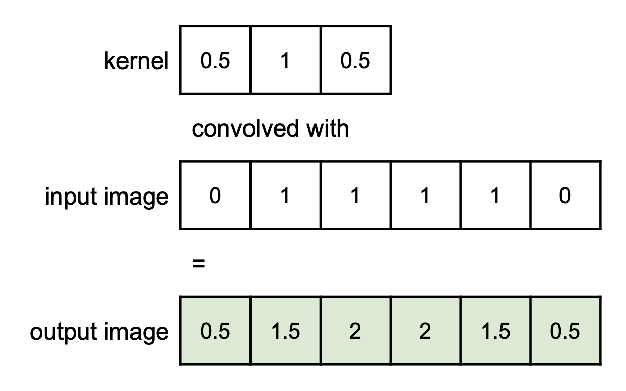
**Figure 1:** 1D arrays representing the input image, kernel, and output image (unfilled).

Answer:

**Figure 1 (ans):** 1D arrays representing the input image, kernel, and output image (filled).

Explanation:

The value of the output image at index is given by the following inner product:

Applying this formula for each index results in the image above.

Convolution over a 2D Image

Suppose that you are given a 1D image vector , representing a 2D image of height and width . You are also given a 1D kernel vector , with radius . You may ignore edges for now.

Write out pseudocode to slide the kernel over the 2D image. At each kernel position, calculate the index of each pixel in the 1D image vector () that the kernel () overlaps with.

Kernel positioned horizontally over a 2D image. — **Figure 2:** An example of a kernel positioned horizontally over a 2D image.

How would you need to adjust this pseudocode if the kernel were positioned vertically instead?

Answer:

For horizontal convolution, the pseudocode might look like this:

for each row in the image...
  for each column in the image...
    for each element in the kernel...
      
      find the row and column of the current pixel:
        row = current row
        column = current column + element index - kernel radius

      use row and column to find the index in the 1D image vector
    
      ...

Continuous Convolution

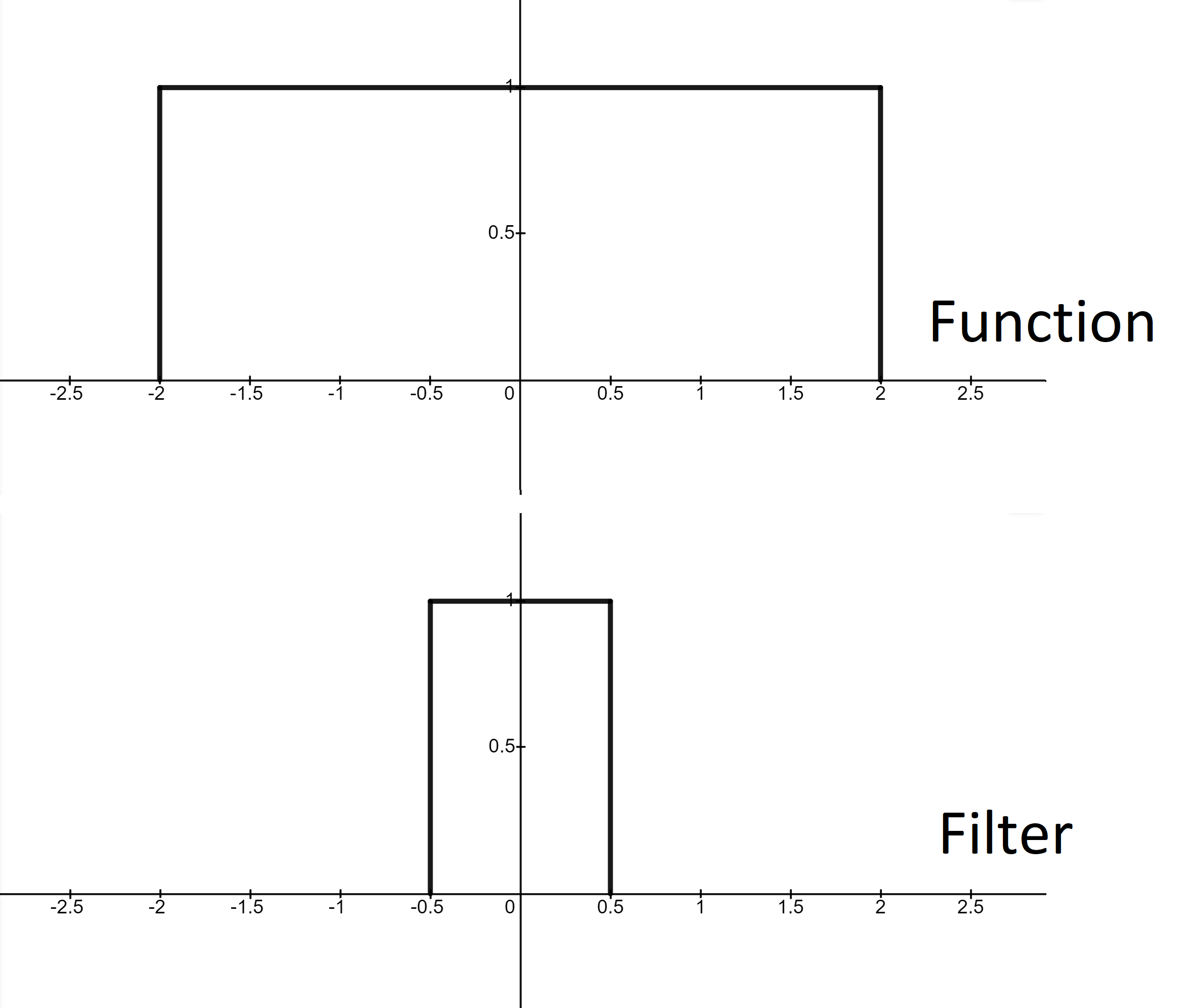
Convolve the below function and filter. What is the value of at in the output?

TODO — **Figure 3:** Image as a continuous signal with filter function for Q1.2

Answer:

. See the next question for the output of the convolution.

Visualizing Convolution

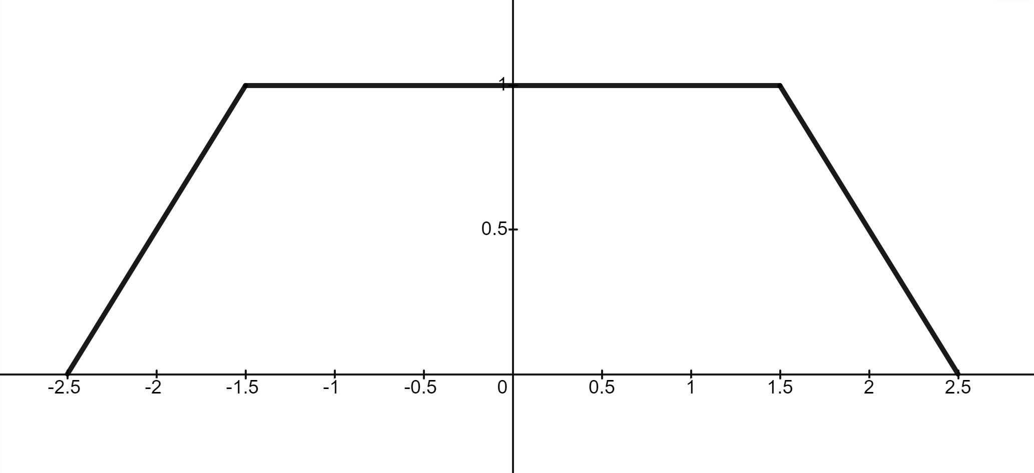
Work with your group on a whiteboard to draw the shape of the output function obtained in the previous question (figure 3).

Answer:

Explanation:

Imagine the filter, flipped (such that becomes ), sliding horizontally across the function.

While doing this, we can identify 4 important points we need to accurately graph the output function:

The first point where the boxes start to overlap (),
The first point where the boxes fully overlap (),
The point where the boxes stop fully overlapping (), and
The point where the boxes stop overlapping at all. (),

As the maximum overlapping area of both inputs is , the maximum value of the output must also be .

From to the output ramps up from to linearly. Then from to the output is constant at . Finally from to the output once again ramps linearly down to . Everywhere else, the output is .

Blurring

Let's try to generalize our solution to the earlier discrete convolution problem.

Consider a 1D kernel of radius that represents a blurring filter. We apply this blur (via convolution) to an input image resulting in a new image .

All of , , and can be considered as 1D arrays storing intensities where gives the intensity of the -th pixel. Remember that the kernel is zero-indexed so gives the left-most value in the kernel array.

We are interested in writing out this convolution as summation over the values of and . For some index within the bounds of the image, please write out the summation equation for in terms of , , , and .

You may ignore edge effects for the purposes of this question (i.e. feel free to "incorrectly" index out-of-bounds).

Begin thinking through this question on your own, and then work with the group to come to an answer. Note that there may be multiple correct answers here!

Answer:

Both answers below are equivalent:

Explanation:

Remember that we must define a summation over the element-wise multiplication of function and kernel , using the kernel's elements .

We must also ensure that is correctly "lined up with" .

With these two constraints in hand, we are ready to define a summation either from to , or from to with different offsets.

Scaling

Scaling Up

What is the filter support width when you scale by a factor of , where ?

Answer

Explanation:

For this explanation, please assume a 1D image.

A triangle filter of width (in units of pixels in the original image) guarantees that, for each output pixel, we are sampling two* pixels in the original image. This effectively performs linear interpolation between the two pixels, and when scaling images, this is usually the way to go (in 2D, it is known as bilinear interpolation).

* Technically...

There are cases where, for an output pixel, we sample only "one" pixel in the original image:

An output pixel at the edge of the image samples only the input pixel at the exact same position, and its neighbor pixel (but with weight 0, since it's at the tip of the triangle);
In fact, any output pixel which has the exact same position as an input pixel will sample only that input pixel, plus its neighbors (again, with weight 0).
- This makes sense, since we already know what color that pixel should be: the same color as the input pixel at the same position.

Scaling Down

What is the filter support width when you scale by a factor of , where ?

Answer

Explanation:

The reason we use a filter while scaling is to avoid aliasing. Ideally, we'd like to use an ideal low-pass filter: this would be a box in the frequency domain, and a sinc in the spatial domain. Of course, we cannot use a sinc, so we approximate this sinc with a triangle (for scaling, in CS 1230).

This approximation is what gives rise to the answer . It can be found in the image processing lecture slides.

Extra: but why is it

It's not necessary for you to understand the math behind this derivation, but given that we have an input image with some max frequency such that (i.e. it obeys the Nyquist limit), we want an output image with max frequency such that:

This corresponds to a filter which looks like a box function with width in the frequency domain. Via an inverse Fourier transform (or simply by Googling it), we can find that its dual in the spatial domain looks like a sinc which first intersects at .

We approximate this sinc with a triangle with width .

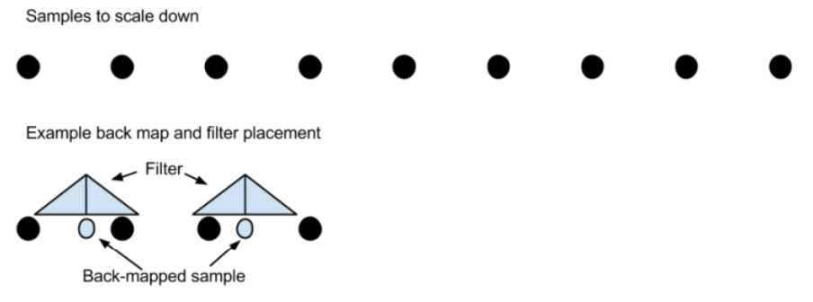
Naïve Back-mapping

Recall from lecture that back-mapping refers to finding the correct filter placement given a pixel in the output image.

The naïve back-map function is $ï$ , but the correct back-map function is , where is the scaling factor and is the pixel index in the output image.

Suppose we wanted to scale down a 9-pixel 1D image by a factor of ().

With your group, draw out the 9 pixels of the original image, and show where we would sample the original image using the naïve back-map function. Include an illustration of the filter above each sample point.

Answer

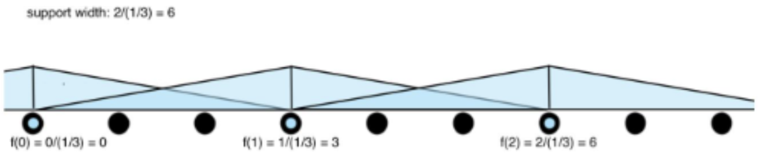
Explanation:

Since we are scaling the image by a factor of , the support width of the filter should be 6. The back-mapping function tells us where to place the filter. For the index of the new image, we need to place our filter at index of the original image. Using the same logic, we place our filter at index 3 and 6 of the original image.

Correct Back-map

Draw another picture to show where we would sample the original image using the correct back-map function. Again, please include an illustration of the filter above each sample point.

Discuss the differences between the two methods, and what might happen if we used the naïve back-map function in practice.

Answer

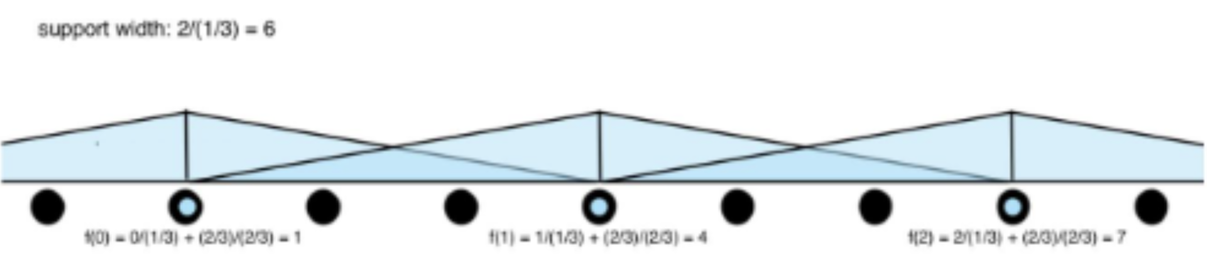
Explanation:

Again, the support width of our filter should be 6 because we are scaling the image by a factor of . The difference between the naïve and correct back-maps is where we place our filter. Using the correct back-map function, we get: index 0 of the new image maps to index 1 of the original image, index 1 of the new image maps to index 4 of the original image, and index 2 of the new image maps to index 7 of the original image.

Duality of Domains

Visualizing Sinc and Box Duals

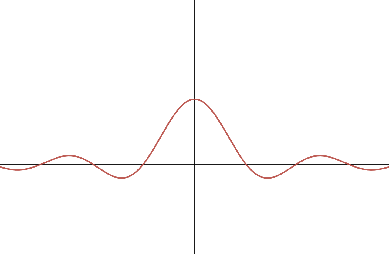
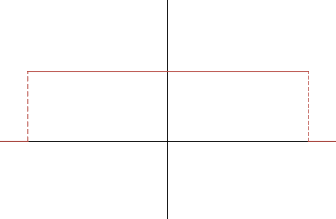
Take a look at the box function in figure 5 (left) below. Its dual in the frequency domain is the sinc function, in figure 5 (right). Note that there are no labels on the axes, by design.

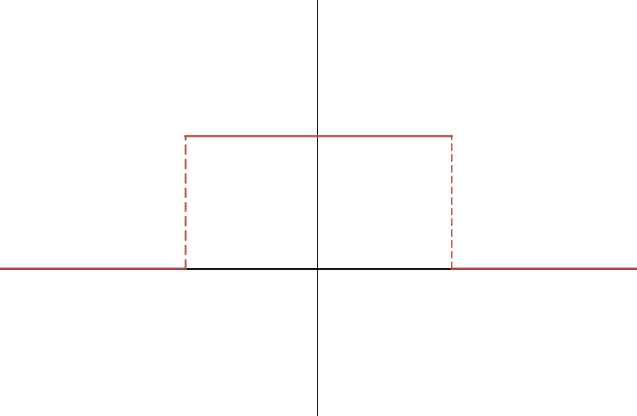
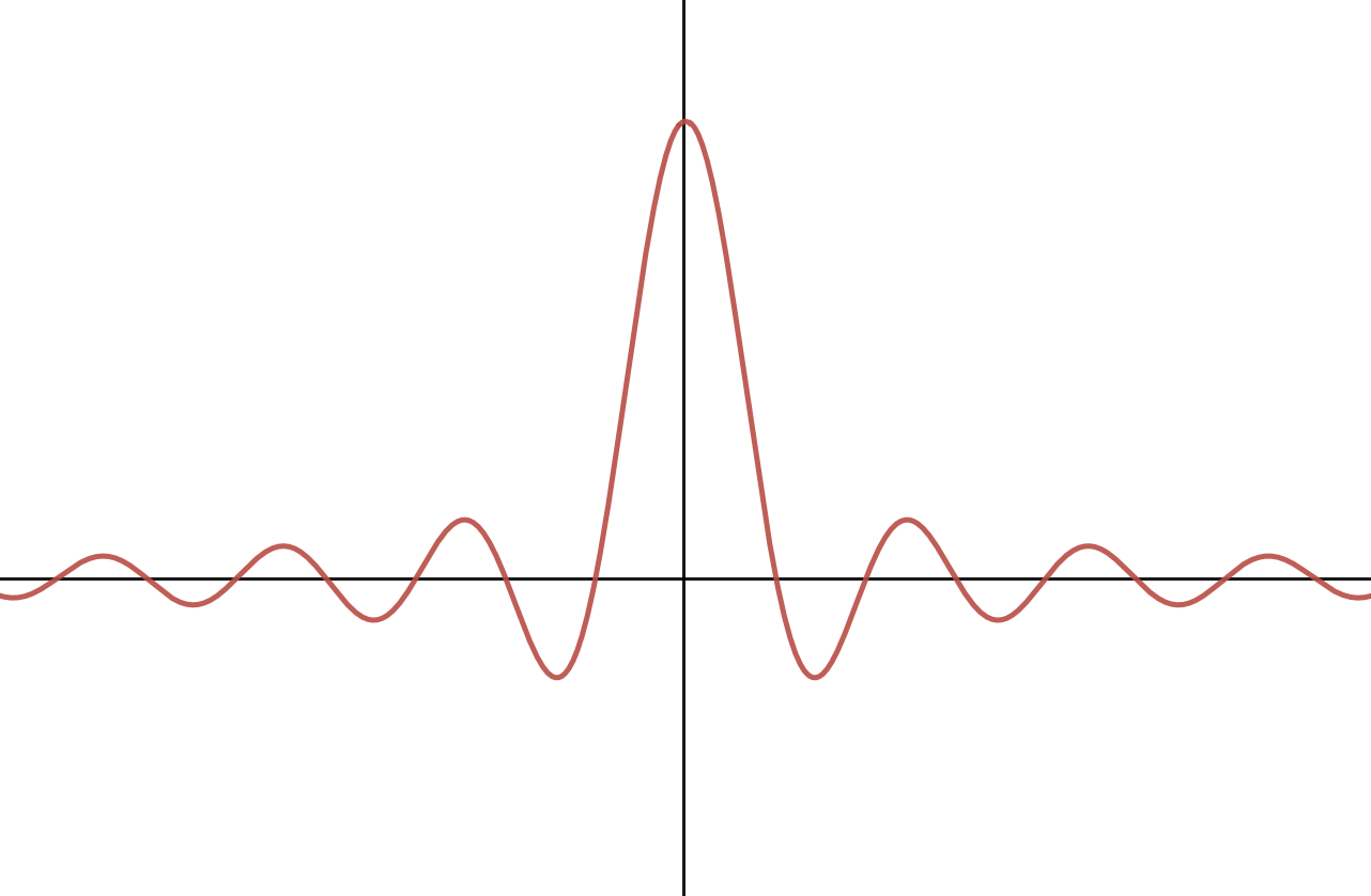
**Figure 5:** A box function with its dual, a sinc function.

A sinc function — **Figure 5:** A box function with its dual, a sinc function.

Draw out a sketch of the dual of the box function in figure 6. Your drawing doesn't need to be perfectly accurate; but enough to show that you understand the concept.

**Figure 6:** Another box function, about twice as wide as before.

When you are finished, explain your group's thought process to the TA.

Answer

Explanation:

A wider box function in the frequency domain means that there are more signals with higher frequency. To reflect this fact in the spatial domain, the sinc function needs to have higher frequency, or, oscillate more. Visually, the sinc function becomes narrower.

Approximating Sinc

What do we usually use to approximate the sinc function, and why do we have to make this approximation when translating these theoretical concepts into code?

Discuss with your group and then call over the TA to check your understanding.

Answer

A Gaussian function. Though, in cases where the approximation doesn't have to be as good, a triangle function can be used instead.

Explanation:

Both the Gaussian and triangle filters are cheaper to use.

Sinc functions are infinite in extent, and it's simply not feasible to perform discrete convolution with an infinitely large, nor would it be performant to approximate it with a "very large" one.

Gaussians are technically also infinite in extent, but fall to almost-zero fairly quickly. Thus, Gaussians can be used as a cheaper approximations to the sinc filter. Compared to the triangle, it also has a nice property: a Gaussian's dual in the frequency domain is another Gaussian, which means it better approximates a good low-pass filter.

Sampling in the Frequency Domain

If we're sampling a continuous function at a frequency of samples per unit, what is the largest frequency we can represent, according to the Nyquist limit?

Answer

Any frequency less than, but not equal to .

Explanation:

In order to capture all frequencies in a signal, we must sample at a rate that is strictly higher than 2 times the highest frequency. Thus, if are sampling samples per unit, we can only represent a continuous function with a frequency of lower than .

Frequency Plots

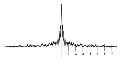
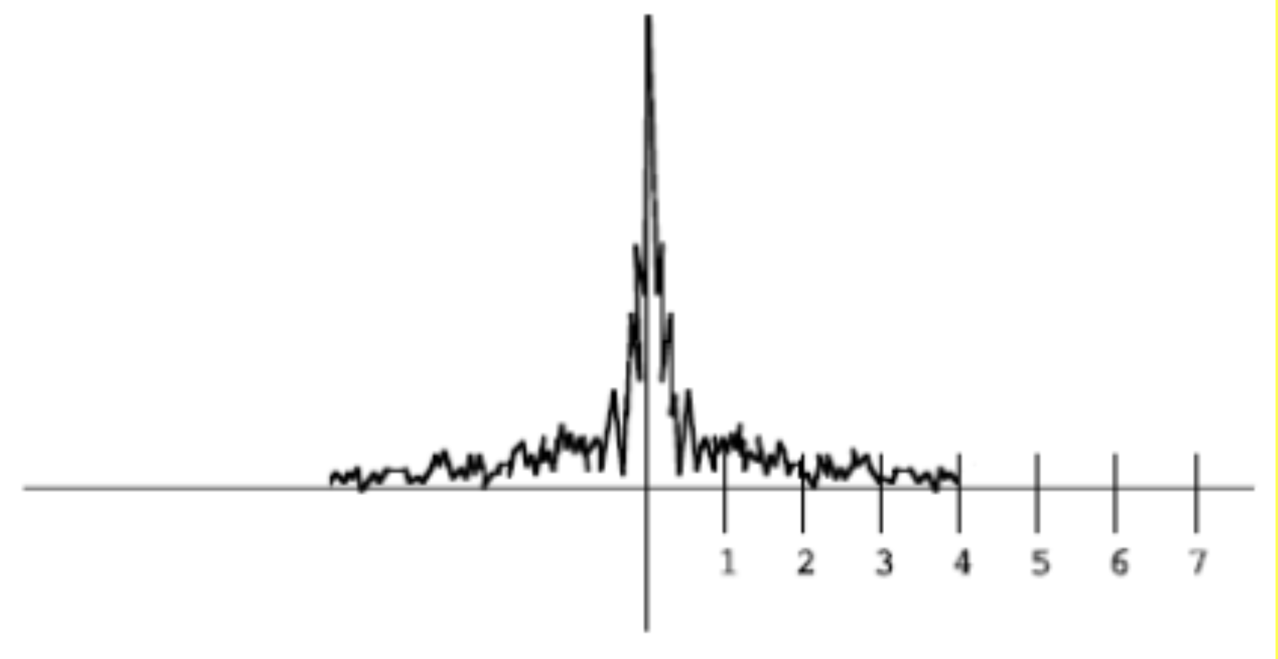
Now, examine the following frequency plot of a 1D, continuous signal. If you were going to sample this signal at a rate of 8 samples per unit, to avoid aliasing, you would use what we know about the Nyquist limit to pre-filter it.

Draw out the new frequency plot after someone has performed this pre-filtering step optimally. Make sure to include any relevant amplitude and/or frequency values.

**Figure 7:** A frequency spectrum. It plots amplitude against frequency.

Answer

**Figure 7 (ans):** A frequency spectrum. It plots amplitude against frequency. This one has been filtered to remove frequencies above 4.

Explanation:

To avoid aliasing, we need to prefilter the signal by running a low-pass (blur) filter to eliminate high frequencies. In the frequency domain, if we want to eliminte frequencies higher than , we can multiply the signal by a box function of width centered around 0. The result is that frequencies under the box are kept.

In our case, since we are sampling the signal at 8 samples per unit, we can only represent functions with frequency lower than 4. Thus, the box function centered around 0 should have width . Frequencies within this box are kept, while higher frequencies are cut off.

Submission

Algo Sections are graded on attendance and participation, so make sure the TAs know you're there!