Lab 3: Transforms and Parsing
Please put your answers to written questions in this lab, if any, in a Markdown file named README.md in your lab repo.
Introduction
Welcome to lab 3! The goal of this lab is to help you get more comfortable with 2D & 3D transformations, coordinate spaces, and scene graphs.
By the end of this lab, you will be able to build transformation matrices, combine them correctly, and then use those ideas while traversing a scene graph to produce renderable data.
Objectives
This lab involves more conceptual understanding than previous ones. Be sure to take your time reading through the sections, and don't be afraid to ask questions if you're confused!
- Learn how matrices are used to represent scaling, rotation, and translation transformations
- Understand how to compose multiple transformations to obtain a cumulative transformation matrix
- Reason about world, object, camera, and local coordinate spaces
- Traverse a scene graph as
SceneData - Convert
SceneDataintoRenderDatafor rendering
Building Transformations
Representing Transformations as Matrices
A transformation can be thought of as a function.
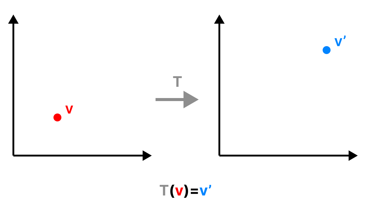
Given an input vector
In 2D,
In 3D,
If
Scaling
Scaling stretches or shrinks an object along each axis. Recall that, to scale
and scale each by the corresponding factor. This produces two new basis vectors:
Therefore, we can construct a transformation matrix for scaling using the basis vectors as the columns. In 2D, the scaling matrix is:
In 3D, the scaling matrix is:
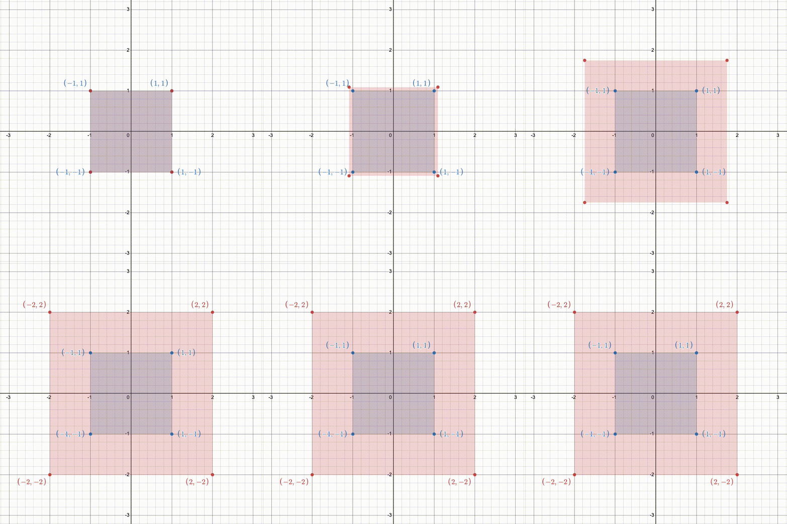
In src/transforms/transforms.cpp, fill in getScalingMatrix so that it returns a 3x3 transformation matrix (as a glm::mat3) based on the three input scale factors.
You may not use any built-in GLM functions for building transformation matrices (namely, scale, translation, or rotate) for tasks 1-8.
How to initialize a glm::mat3
The most useful ways to construct a matrix in glm are:
glm::matN(float x)initializes anNxNmatrix withxalong the diagonal. Example:glm::mat3(2.0f)produces. glm::matN(float x_11, ... float x_nn)initializes all values explicitly in column-major order.glm::matN(glm::vecN v_1, ... glm::vecN v_n)uses the vectors as columns.
glm uses column-major order, so be careful when specifying values directly.
Rotation
Rotation turns an object about the origin. We can rotate the standard basis vectors
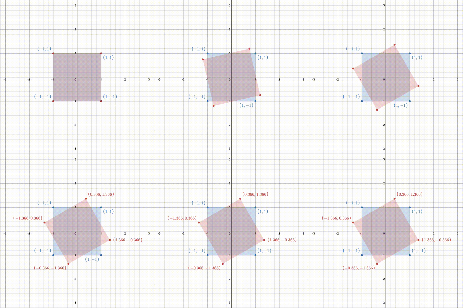
In 3D, this is a bit more complex. Rather than always rotating CCW about the origin, 3D allows for rotation around any arbitrary axis.
There are many ways to describe rotations in 3D (as covered during the lectures), but we'll use the axis-aligned Euler angles approach as this is the simplest for when we construct our own matrices.
For this, we define 3 rotations, one about each standard axis, and then compose them in a specified order. We use
Fill in getRotationMatrixX, getRotationMatrixY, and getRotationMatrixZ so that each returns the 3x3 matrix that rotates about the named axis by the given angle.
Notes and useful functions
These functions might be useful, and you can use glm::radians to convert angle units.
Note: glm and the <cmath> library expect radians angle units.
Also remember that glm expects column-major order during initialization.
3D rotation about arbitrary axes requires composing the above individual transformations. One common approach is to multiply the
To transform
Such that:
Pay attention to the sequence of multiplication that
Translation and Homogeneous Coordinates
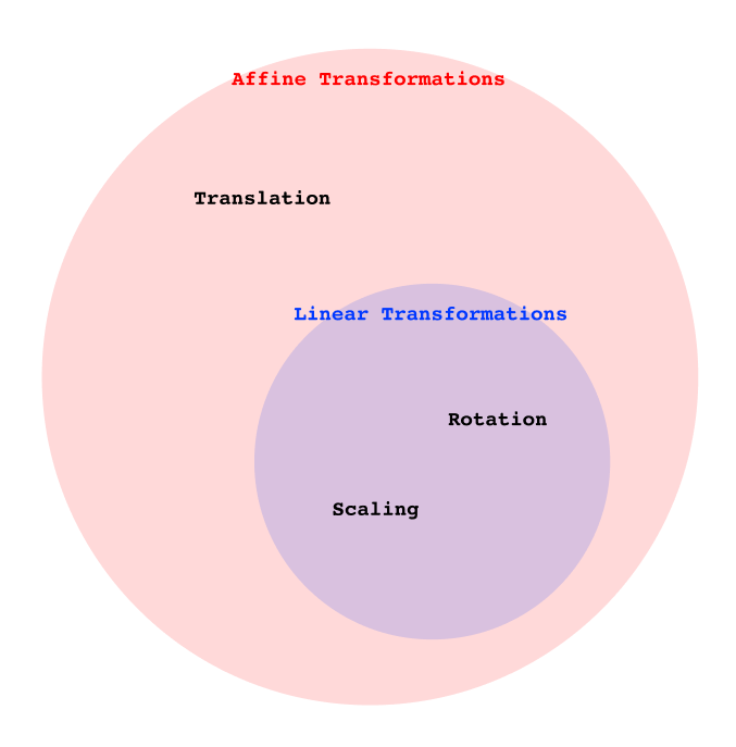
Translation moves a point without changing its shape or orientation. Unlike scaling and rotation, translation is not linear, it is an affine transformation.
Generally speaking, linear transformations are a strict subset of affine transformations.
Extra: more information about transformation classification
There are many ways to classify transformations. In the paragraphs above, we are considering their mathematical formulation: translation is not a linear transformation as it does not preserve the origin, and this conclusion is entirely based on the definition of what a linear transformation is.
You will soon see that what is non-linear in one dimension, can actually be linear in a higher dimension 😉.
There is, of course, another way to look at classify transformations. We might do so based on what geometric features they preserve:
Type Of Transformation What They Preserve Examples Displacements Distances and oriented angles Translations Isometries Distances and angles Rotations, reflections, and the above Similarities Ratios between distances and angles Uniform scaling, and the above Affine transformations Parallelism Non-uniform scaling, shear, and the above Projective transformations Collinearity Perspective projection, and the above Adapted from the Wikipedia page on geometric transformations
Illustration of the problem we now face
To illustrate the problem we are now facing, suppose we wanted to translate points by some non-zero vector
Oh dear. No matter what values we put in 2x2 matrix, the output can never be equal to non-zero vector 2x2 matrix is not sufficient for representing a translation of a 2x1 point in this way (and the same can be shown for 3x3 matrices, with 3x1 points).
If we wish to represent translations as matrices, we must now introduce homogeneous coordinates.
Homogeneous Coordinates
While homogeneous coordinates are pretty simple to use, they might be somewhat challenging to understand. The idea is this: take any existing point or vector, and just add another dimension to it. Then, do the same for transformation matrices.
In 3D, for example, this turns a 3x1 point into a 4x1 point. We typically refer to this new, fourth dimension as
For points (position vectors), we set
Reminder: points vs. vectors
A point is characterized by having a specific position in space.
A vector has a magnitude and a direction, but no location.
One way to think of this mathematically is that a vector is the difference between two points, like the displacement from one to the other. It doesn't matter where it starts and ends. Conversely, points only have a location, but no sense of size or orientation.
In 2D, points become
In 3D, we get:
- points become
- vectors become
Extra: how does this affect what we've learned so far?
Fortunately, adding the extra dimension does not break how points and vectors work. We won't prove this, but here are two examples:
But, we'll have to modify our previous linear transformations to be compatible with our new matrix size. For scaling and rotation, we simply add another dimension (i.e. another row and column) with
Note how the new, "extended" portion of the matrix resembles the identity matrix. Intuitively, this is because we do want our transformation matrix to still do the same thing, and not change its behaviour just because we added another dimension.
As mentioned earlier, we must also enlarge our transformation matrices: in 2D, they become 3x3; and in 3D, they become 4x4. The translation matrix in 3D can now be expressed as follows:
See how adding the
Example: attempting to translate vectors
Since
Now that we know how to perform translation in n dimensions by using an (n+1)x(n+1) matrix, here's an example to tie it all together:
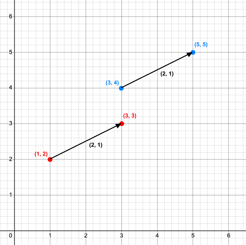
Fill in getTranslationMatrix() so that it returns the 4x4 transformation matrix (as a glm::mat4) that translates along each axis by the given coordinates.
Then update getScalingMatrix(), getRotationMatrixX(), getRotationMatrixY(), and getRotationMatrixZ() to work with homogeneous coordinates so they return glm::mat4s instead of glm::mat3s. Do not forget to update the headers in transforms.h.
Applying Multiple Transformations
Being able to apply only a single transformation would probably make it hard to create interesting scenes unless your goal is to make a brick wall. We can apply multiple transformations by composing them. Mathematically, this is represented by multiplying the respective matrices in the order that the transformations are applied.
If we have two transformations
Due to the associativity of matrix multiplication, we can multiply
Important: Matrix multiplication is not commutative, so changing the order changes the result.
Ordering (S)cale, (R)otation, and (T)ranslation
If you have one object that you want to apply multiple individual scale, rotation, and translation transformations to, you should be careful of the order in which you compose the transformations. Usually, you want to use a standardized order in which you apply transformations to maintain consistency.
One widely used ordering is TRS. This means that scaling is first, then rotation, then translation.
Why TRS ordering works
Let's say we have a square at the origin that we want to perform the following transformations on:
- Scale x by 1.5 and y by 2
- Rotate by 45°
- Translate by (3, 3)
Here's what happens if we translate, then rotate, then scale (SRT):
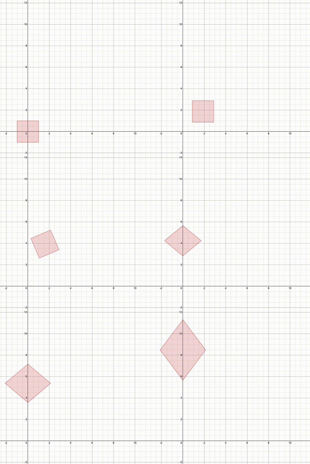
Notice how we scale along the standard axes, so rotating first changes the way the object is stretched. Both rotation and scaling are centered at the origin, so translating first changes the final position.
And here's what it looks like if we scale, then rotate, then translate (TRS):
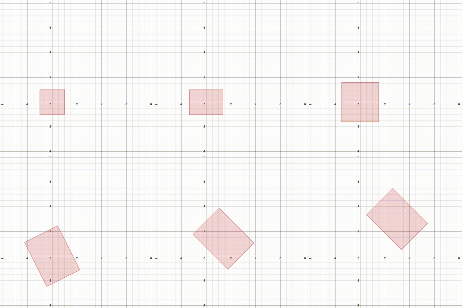
Which looks more like the result you'd expect?
Scene Graphs And Cumulative Transforms
Now that you know how to build and compose transforms, we can use them on a scene graph.
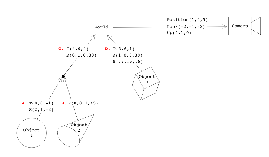
There are a lot of different parts of this graph to understand, but for now let's focus on some of the labeled transformations. A, B, C, and D all denote individual transformation matrices that involve some combination of scaling, rotating, and translating.
How to read the transformations
At the top of the graph is the world origin. From it, the rest of the objects and camera branch off, with nodes in between to represent the transformations applied to the objects and camera.
Here's a guide to our notation of transformations:
S X,Y,Z:   scale by factors X, Y, and Z along the corresponding axes
R X,Y,Z,𝜃: rotate by angle 𝜃 about the axis defined by unit vector [X,Y,Z] ([1, 0, 0] would denote the x-axis, for example)
T X,Y,Z:   translate by X, Y, and Z along the corresponding axes
Fill in functions getMatrixA, getMatrixB, getMatrixC, and getMatrixD using the functions you defined in Tasks 1-4 to return the matrices corresponding to the transformations described in the graph.
In a scene graph, a node's transforms apply to everything below it. To find the final transform for an object, multiply the transforms along the path from the root to the node that contains that object.
That final product is the object's cumulative transformation matrix, or CTM.
How to think about the traversal
Looking at our graph again, each leaf of the tree is an object in the scene. Traversing the tree from the object to the root will create a path through all of the transformations applied to that object in the scene. So to transform Object 1 to world space, for example, first apply transformation A then C. The cumulative transformation matrix of an object in the scene, resulting from this ordered multiplication of matrices, is referred to as the object's model matrix.
Previously, we emphasized the need to order each of the T, R, and S transformations. Now we may be dealing with multiple matrices composed of multiple T, R, and S transformations, but for the higher level ordering we follow the graph hierarchy.
Demo And Inverse Rotation
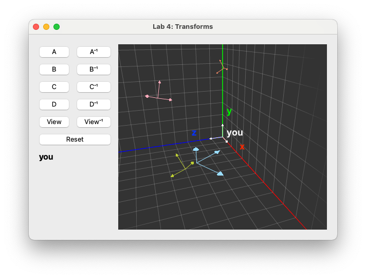
To help you check your work, the stencil includes a visualizer that lets you apply the transformation matrices from the graph.
How to use the demo
You can click and drag to move around and scroll to zoom.
The white grid in the background represents the world coordinate system. The white axes at the origin represent your current coordinate system. Though they aren't labeled in the demo, these are labeled here for your reference.
Each of the buttons A, B, C, and D are linked to the functions you completed in the last task to return transformation matrices. Pressing any of these buttons will apply the corresponding function's transformation to the white axes. We have also provided you with inverse buttons for each of these that will return the inverse of the corresponding matrix. (Don't worry about the "View" or "Rotation" buttons for now, you'll be implementing those later.)
As you press the buttons, the text underneath that says "you" will update to reflect the order of transformations you use. Pressing the "reset" button will move your axes back to the origin and reset this label.
Having issues running your code?
If you run your code and don't see the axes, or if your program immediately crashes with an error along the lines of
terminating with uncaught exception of type std::runtime_error: Failed to open shader: resources/shaders/grid.vert
this is for you!
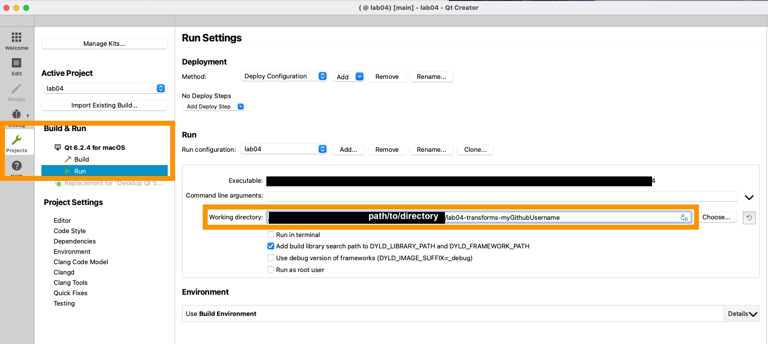
On the left side of Qt Creator go to the Projects > Run menu and check your working directory. Ensure that the listed filepath is the absolute path to the root folder of the lab git repo. The most likely issue is that the program is unable to load the shader files we use for rendering the scene because the filepaths are relative to the root directory!
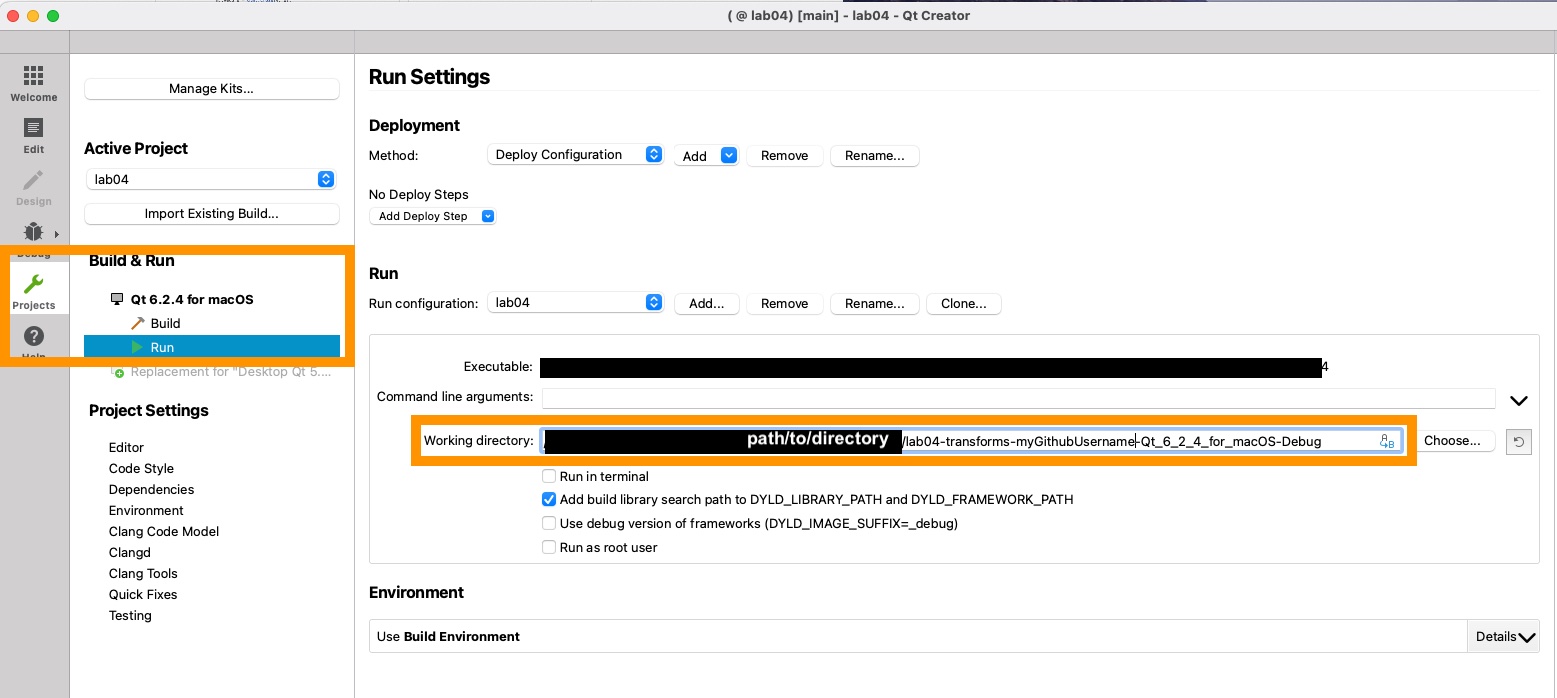
Correct:
There are colored sets of axes throughout which represent the coordinate systems of the different objects in the scene as described in the graph. These are not labeled because it will be up to you to figure out which belongs to which object.
Use the A, B, C, and D buttons to transform the white axes from the world origin to the coordinate system of each object represented by the colored axes. Your task is to find the transformations for Objects 1, 2, and 3 given in the scene graph and find which colored axes correspond to each object.
Note: You will only end up matching 3 of the 4 colored axes. The fourth is for a later task.
Hint
You can think of the white axes as starting in each object's object space, and your goal is to follow the transformation graph to transform it into world space.
If you have implemented your matrices correctly and apply them in the correct order as described in the provided transformation graph, you should see the white axes line up with another colored axes.
Note: Each colored axes is an object from the transformation graph. This means it may or may not require multiple transformations to reach it. Using the transformations you created, you should be able to match 3 of the 4 colored axes. We recommend rereading the paragraphs above this task if you are confused.
As a quick debugging exercise, the stencil also includes an inverse rotation function called getInverseRotation(). The function relies on the useful fact that the inverse of a rotation matrix is its transpose. However, it currently has a bug 🐛
- Press the
Rotationbutton in the visualizer.- This function is already implemented and rotates your coordinate space about the vertical axis by a small angle.
- Press the
Rotation^-1button (which callsgetInverseRotation). Does it apply the transformation you expect it to? - Identify and fix the bug in
getInverseRotation().
Note: You may not use
glm::inverseorglm::transposeto implement this function.
Verify that Rotation followed by Rotation^-1 returns the axes to their original state.
Camera View Matrix
The camera's placement in world space is described by a position and orientation. A key part of rendering is showing the scene from the camera's point of view. To do so we use the inverse of the camera transform. That inverse is the view matrix. By applying the view matrix to all points in the scene, we transform them from world space into camera space, and thus the camera's point of view.
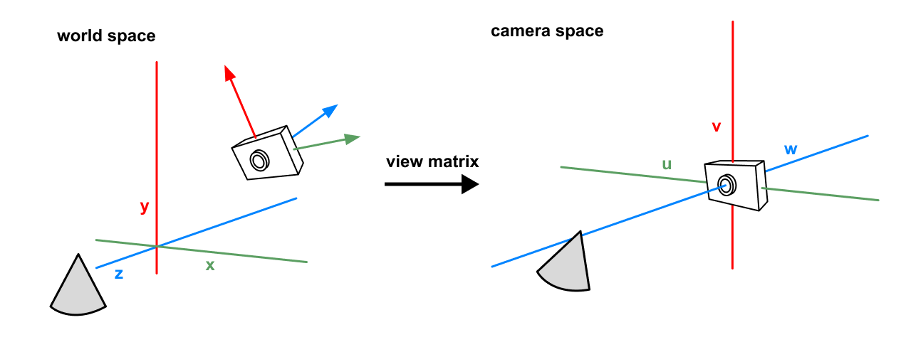
The camera is defined by its position
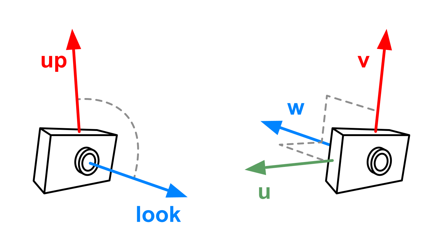
(Note that look and up are not always orthogonal but that calculating uvw accounts for this.)
From those, we compute the camera axes
The view matrix is made from a translation that moves the world by
Finally, putting the rotation and translation together, we get one matrix for transforming other objects into the camera's coordinate system.
Wait, why T then R?
Wondering why our view matrix does translation first and then rotation, even though earlier we said rotation should usually come first?
As with the objects' model matrices that we looked at previously, the matrix that transforms the camera to world space is composed of a rotation first then a translation. Since the view matrix is the inverse (it transforms objects from world space to camera space), we must reverse the order of the multiplication.
Fill in getViewMatrix in src/transforms/transforms.cpp to return the camera's view matrix using pos, look, and up.
These functions might be helpful for working with vectors.
If you run the demo again now you should be able to use the "view" button to apply the view matrix transformation. Careful though! Remember that the view matrix transforms the world coordinates to the camera coordinates (note the direction of the arrow in the graph). If you want to view the transformation of the camera coordinates to the world coordinates (i.e. moving your white axes from the origin to the camera's axes in the demo), which button should you actually press?
Coordinate Spaces
In discussing transformations, we've mentioned the idea of transforming between coordinate spaces, but what are coordinate spaces? This is an important concept as you work on building your raytracer. You will often find that certain calculations make sense when you work with them in specific coordinate spaces, but when you're dealing with points and vectors in different spaces you need to know how to use transformations to move between them.
In this lab, we use three coordinate spaces often: world space, camera space, and object space.
- World space is the global coordinate system for the scene.
- Camera space is the coordinate system defined by the camera.
- Object space is the local coordinate system in which a single object is defined.
Extra: more info on coordinate spaces
World Space:
Think of world space as your default overarching coordinate system. Everything else gets placed into the scene relative to the origin and units of the world's coordinate system. World space is arbitrarily defined and acts as a fixed space within which everything else can be defined. In the transformation graph we've been looking at, it is the root that everything else stems from.
Camera Space
Camera space is what you learned about in part 2.9 of this lab. It is the coordinate system defined by the camera's position and rotation. In camera space, everything else in the world is relative to the camera's view, with the camera being placed at the origin, and its
Object Space
Object space is pretty much what it sounds like - the coordinate system in which an object is defined. In the demo, these are represented by the little sets of axes drawn for each object in the scene.
Why do we need coordinates specific to each object?
For example, you might want to make a bunch of variations of a sphere that are all different sizes and in different locations. Rather than define each sphere separately, we can define a single sphere as a set of points around an origin, and then transform those points. You can perform calculations on points in the sphere relative to its own central origin, and then use its model matrix to get those points in world space.
Relating All Three
Here's a simpler graphic that helps to sum up the relationships between everything we covered so far in this lab.
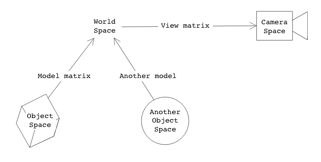
The arrows indicate the direction of transformation that the labeled matrix provides. An object's model matrix will convert from that object's space to world space. The view matrix will convert from world space to camera space. The inverses of these matrices provide the transformation of the opposite direction.
Consider the following situation where you have a scene with a camera, a cube, and a light as such:
You know the coordinates of point
Your response should be no more complex than just stating "multiply __ and __ to get __ in ______ space. Then..."
Scene Data and Render Data
Scene Data vs. Render Data
We have spent most of this lab building and composing transformation matrices. Now we use those ideas to understand how a scene file becomes renderable data, and ultimately cool 3D scenes.
SceneDatais the tree-based representation used while building a scene, known as a scene graph.- This is often arranged in a tree structure that groups logical (and often spatial) relationships between objects in the scene.
RenderDatais the flattened representation used while rendering.- In
RenderData, each object/primitive stores its final cumulative transform, so the renderer no longer has to traverse the scene graph.
- In
Take a look at the two figures below. In this lab, your task will be to write a parser which transforms SceneData to RenderData.
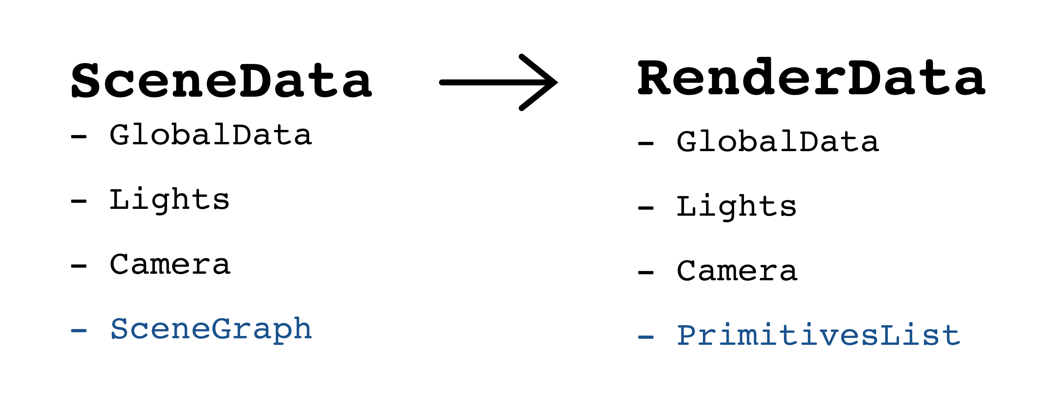
Transforming SceneData into RenderData. Conceptually, they store the same information, just in a different format!
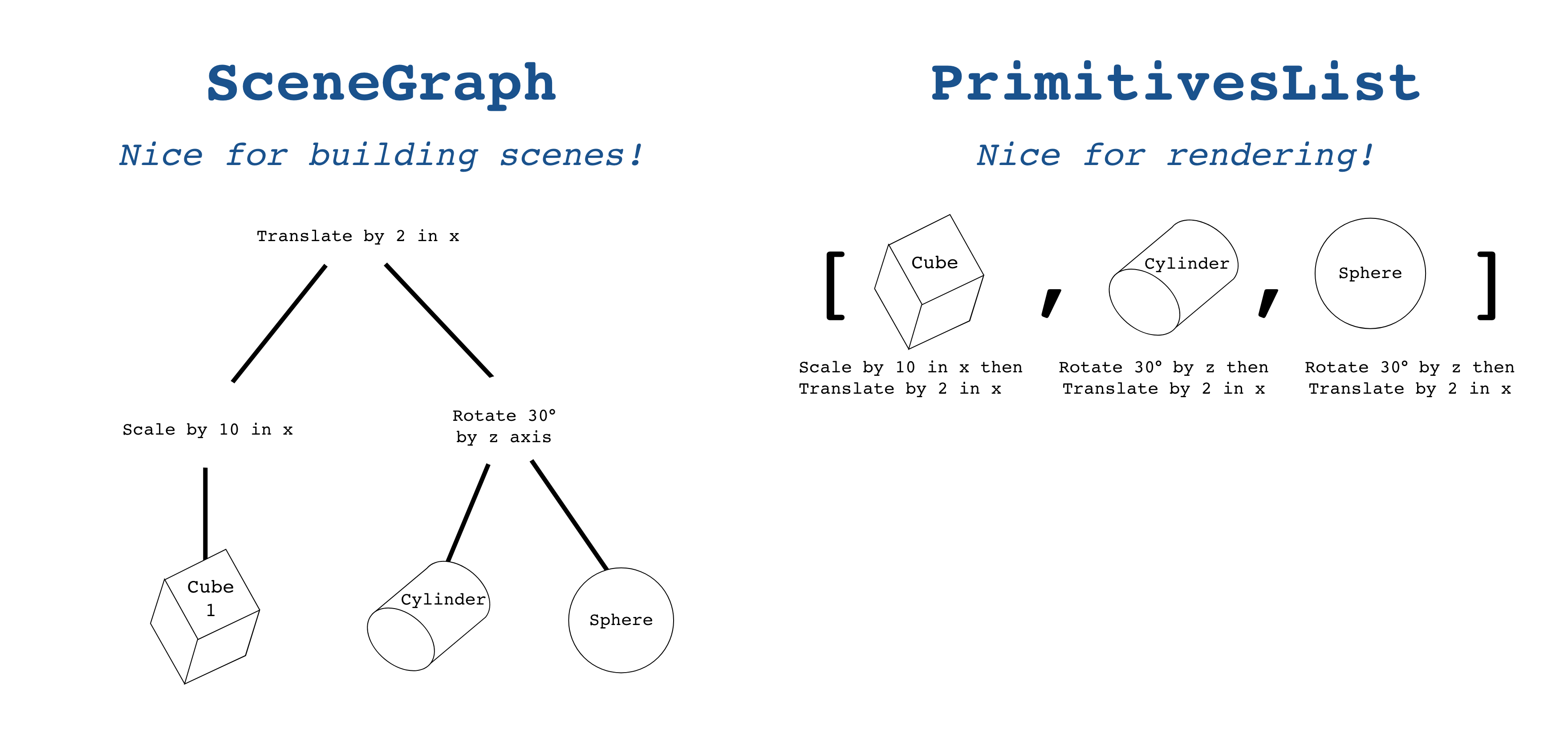
In Figure 17, observe how the SceneGraph and PrimitivesList are the only things that differentiate SceneData from RenderData. Figure 18 shows how primitives and their transformations are stored differently in these data structures.
Extra: why do we use a vector/list to store primitives?
If you have started Project 2: Intersect, you might have reasoned that one of the reasons ray tracing is so computationally expensive is because we need to check for ray-primitive intersections. This is especially true when there are many primitives in the scene to check against.
We use a vector/list to iterate through all the primitives in the scene because it is simple to implement, and has traditionally been sufficient for the requirements of this course.
That said, there isn't any reason that this part of RenderData has to be a vector/list. If you want to get fancy, there are more efficient alternatives which allow for much faster ray-primitive intersection tests (see: "accelerated" data structures like octrees, bounding-volume hierarchies (BVHs), and KD-trees, all covered in lectures).
Scene Data
The parser gets the data it needs from ScenefileReader with relevant information found in src/parser/SceneData.h. The important pieces are:
SceneGlobalData, which stores the global shading coefficients, essentially denoting how light interacts with the scene. You will learn more about these later in the course.
Extra: more info
// Struct which contains the global color coefficients of a scene.
// These are multiplied with the object-specific materials in the lighting equation.
struct SceneGlobalData  {
    float ka; // Ambient term
    float kd; // Diffuse term
    float ks; // Specular term
    float kt; // Transparency; used for extra credit (refraction)
};
SceneGlobalData stores the global ambient, diffuse, and specular coefficients, as well as the transparency index of refraction. These are used to calculate how light interacts with the scene.
SceneCameraData, which stores the camera position, look, up, and field of view.
Extra: more info
// Struct which contains data for the camera of a scene
struct SceneCameraData {
    glm::vec4 pos;
    glm::vec4 look;
    glm::vec4 up;

    float heightAngle;   // The height angle of the camera in RADIANS

    float aperture;      // Only applicable for depth of field
    float focalLength;   // Only applicable for depth of field
};
SceneCameraData stores pos, look, and up in world space, so the view matrix can be built directly from those values. One important thing to note is that pos, look, and up are all defined in world space. They'd be pretty useless if they were defined in camera space.
SceneLightData, which stores the scene lights.
Extra: more info
SceneLightData supports point, directional, and spot lights. A point light has a position. A directional light has a direction. A spot light has both, plus cone parameters.
// Struct which contains data for a single light
struct SceneLightData {
    int id;
    LightType type;

    SceneColor color;
    glm::vec3 function;  // Attenuation function

    glm::vec4 pos;       // Not applicable to directional lights
    glm::vec4 dir;       // Not applicable to point lights

    float penumbra;      // Only applicable to spot lights, in RADIANS
    float angle;         // Only applicable to spot lights, in RADIANS
};
Each light in our scene is represented with a struct that includes its LightType, its color, and other relevant information depending on the LightType.
- A point light is a single point in space that emits light equally in all directions (e.g. an infinitesimally small lightbulb). It is defined by its color and position.
- A directional light is a global light which simulates light from a source that is infinitely far away (e.g. the sun, as we experience it on earth). It is defined by its color and direction.
- A spot light is much more interesting—it is effectively a point light, but it emits light only in a cone shape (e.g. a flashlight). It is defined by its color, position, and direction, as well as a penumbra and angle, which describe its cone.
Documentation about virtual lights commonly used in 3D scenes can be readily found online, such as in the Unity3D manual.
ScenePrimitive, which stores the primitive type, material, and optional mesh file.
Extra: more info
ScenePrimitive stores the primitive type and material. Mesh files are only needed for triangle meshes.
// Enum of the types of primitives that might be in the scene
enum class PrimitiveType {
    PRIMITIVE_CUBE,
    PRIMITIVE_CONE,
    PRIMITIVE_CYLINDER,
    PRIMITIVE_TORUS,
    PRIMITIVE_SPHERE,
    PRIMITIVE_MESH
};
Much like with LightType, we use PrimitiveType to identify different types of primitives. This is used in a struct, ScenePrimitive, to describe a specific primitive in the scene:
// Struct which contains data for a single primitive in a scene
struct ScenePrimitive {
   PrimitiveType type;
   SceneMaterial material;
   std::string   meshfile; // Used for triangle meshes
};
Every primitive has both a type and material. The meshfile field will only be relevant if you'd like to implement triangle mesh rendering, an extra credit option for our Ray and Realtime projects.
material contains important information about what the primitive looks like (e.g. its color, how shiny it is, any textures, etc.). You can look at the definition of SceneMaterial for details, but it's fine not to understand any of the terms which haven't yet been covered in lecture.
Observe that, unlike the light or camera structs, there aren't any fields in ScenePrimitive that describe its transformation. This is because it's more practical to use scene graphs to manage this, especially when we have a lot of primitives!
SceneTransformation, which stores translate, scale, rotate, or matrix transforms.
Extra: more info
The parser uses four types of transformations:
// Enum of the types of transformations that can be applied
enum class TransformationType {
    TRANSFORMATION_TRANSLATE,
    TRANSFORMATION_SCALE,
    TRANSFORMATION_ROTATE,
    TRANSFORMATION_MATRIX
};
SceneTransformation stores the specific data for one transform:
// Struct which contains data for a transformation.
struct SceneTransformation {
    TransformationType type;

    glm::vec3 translate; // Only applicable when translating.
    glm::vec3 scale;     // Only applicable when scaling.
    glm::vec3 rotate;    // Only applicable when rotating.
    float angle;         // Only applicable when rotating.
    glm::mat4 matrix;    // Only applicable when transforming by a custom matrix.
};
SceneNode, which stores a list of transformations, primitives, and child nodes.
Extra: more info
Our scene graph is composed of nodes, each of which describes zero or more of the following:
- a series of transformations,
- a number of primitives, and
- a number of child nodes.
SceneNode looks like this:
// Struct which represents a node in the scene graph/tree, to be parsed by the student's `SceneParser`.
struct SceneNode {
   std::vector<SceneTransformation*> transformations; // Note the order of transformations described in part 4.3
   std::vector<ScenePrimitive*>      primitives;
   std::vector<SceneNode*>           children;
};
If a SceneNode has transformations, those apply to both its primitives and children.
Scene Graphs
Recall from earlier that the CTM (cumulative transformation matrix) of a primitive is the ordered product of all transformations from the root down to that primitive's node.
Earlier, we chose TRS ordering when composing transformations. Here, the scene file has already fixed an order for each node.
Multiply transformations into the CTM in list order:
node.transformations = [t1, t2, t3]
ctm = ctm * t1 * t2 * t3
Because of how matrix-vector multiplication associates, this means the last transformation is actually applied to a point first, and the first one last.
Implementing SceneParser::parse()
Whenever we load a scene, we call SceneParser::parse() (located in src/parsing/sceneparser.cpp) to convert the scene data into render data.
bool SceneParser::parse(std::string filepath, RenderData &renderData) {
    ScenefileReader fileReader = ScenefileReader(filepath);
    bool success = fileReader.readJSON();
    if (!success) {
        return false;
    }

    // Tasks

    return true;
}
The first step is to copy the global and camera data from fileReader into renderData.
Use the fileReader methods to assign the scene's global data and camera data into renderData.
Traversing The Scene Graph
The next step is to traverse the scene graph, build cumulative transforms, and populate renderData.shapes and renderData.lights.
Instead of walking back to the root every time we need a CTM, it is more efficient to build the cumulative transform as we descend the tree. That means passing the current transform down to each child and updating it as we go.
This is a much bigger task than the others in this lab. If you get stuck, remember that you can collaborate with others in this course!
Start by getting the root node from fileReader and clearing renderData.shapes.
Then perform a depth-first traversal of the scene graph. As you traverse, keep a running cumulative transform. For each primitive you encounter, create a RenderShapeData with that primitive and its CTM, then append it to renderData.shapes.
For each light you encounter, construct a SceneLightData and append it to renderData.lights. Light positions should be transformed as points, and directions should be transformed as vectors, both into world space.
Use a recursive helper if that makes the traversal cleaner. Think carefully about which values should be passed by reference and which should be passed by value.
Note: Scene file rotations are specified as an arbitrary axis (
glm::vec3) and angle (given to the program in radians), not necessarily aligned to X, Y, or Z. Your earliergetRotationMatrixX/Y/Zfunctions will not work for this purpose. You are allowed and encouraged to use the built-inglmfunctions for building transformation matrices. You may findglm::translate,glm::scale, andglm::rotateuseful for building the matrices for each transformation.
Testing Scenes
Once your parser is wired up, you should be able to load scenefiles like directional_light_1.json, ambient_total.json, and primitive_salad_1.json (all located in resources/scenefiles/).
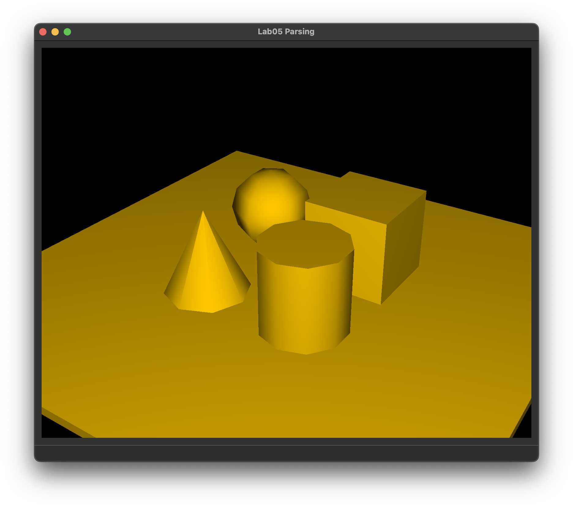
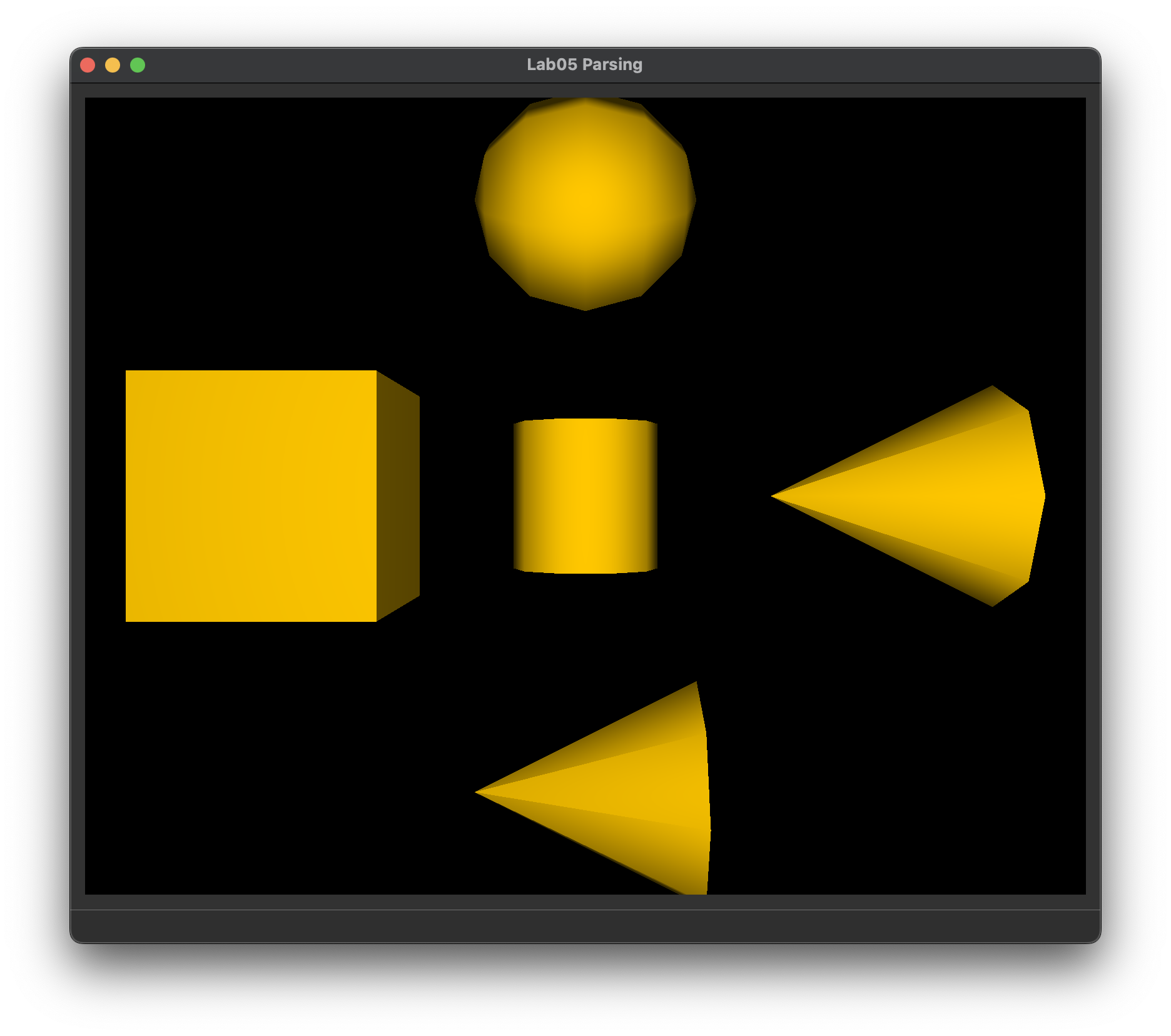
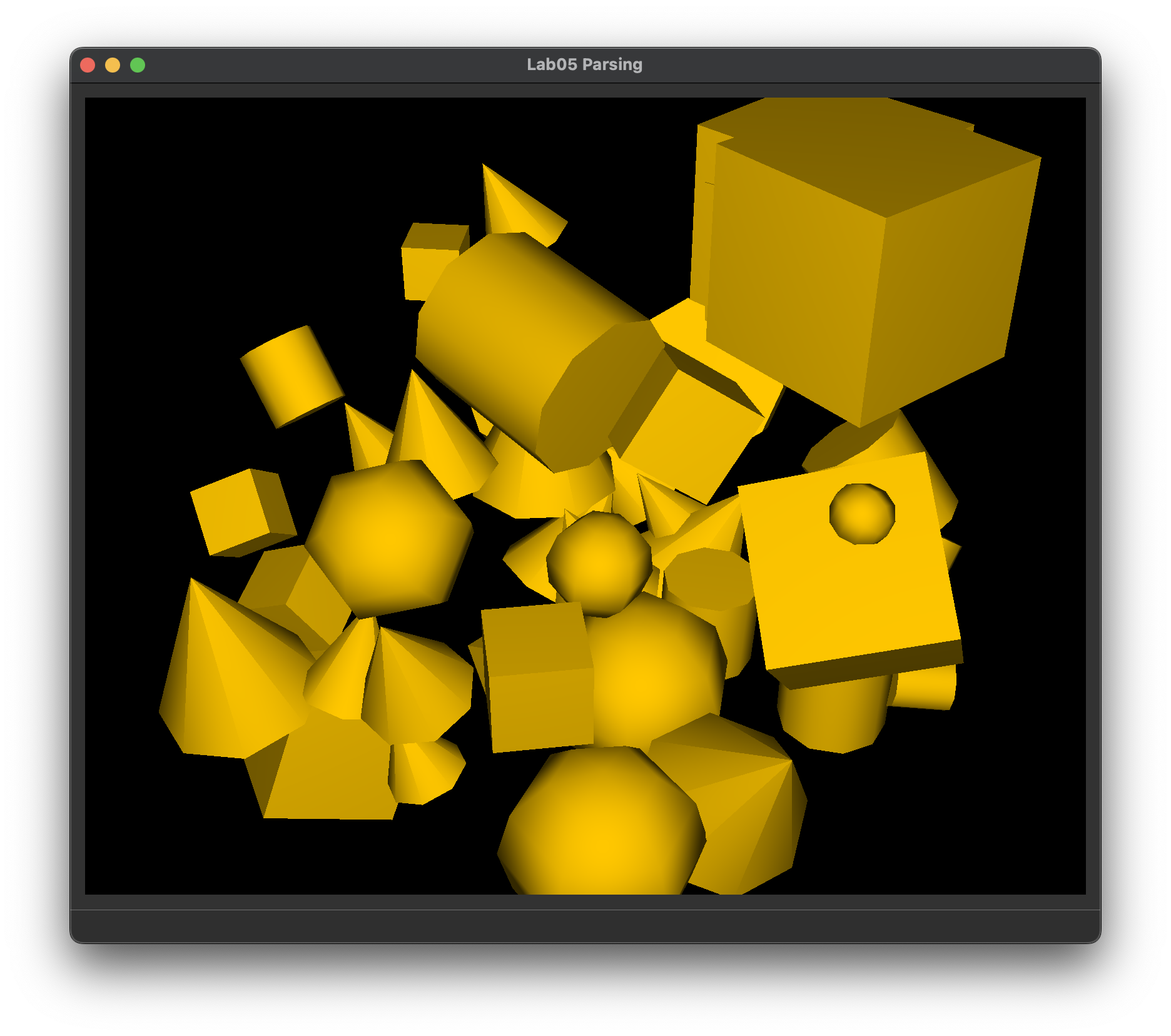
Loading a scene helps verify that the camera, primitives, and transformations are correct. The lighting support code is intentionally basic, so this does not fully validate every light-related detail.
End
Congrats on finishing the transforms and parsing lab! By this point, you should be able to explain the transformation rules, the camera view matrix, and how a scene graph becomes render data.
Submission
Submit your GitHub link and commit ID to the "Lab 3: Transforms & Parsing" assignment on Gradescope, then get checked off by a TA at hours.
Reference the GitHub + Gradescope Guide here.