Lab 8: Trimeshes

Github Classroom assignment

Please put your answers to written questions in this lab, if any, in a Markdown file named README.md in your lab repo.

Introduction

Welcome to lab 8!

At this point in the semester, you must've had some experience with implicit shapes. These represent surfaces via a set of constraints (i.e. equations and inequalities), such that all points which satisfy these constraints lie on the surface of the shape. That's rather indirect!

In this lab, we will learn a different representation of surfaces—triangle meshes, or trimeshes for short—which more explicitly describes points on a surface. We will spend some time today understanding what they are, how they work, and how we can generate our own.

Objectives

Learn about trimeshes and how they are used to approximate an object's surface;
Implement generators for cube, sphere, and cone trimeshes at varying levels of detail.

Conceptual Background

Objects As Trimeshes

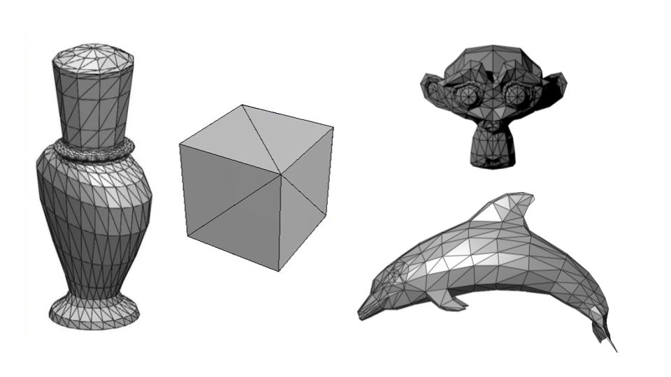
Most objects can be represented as surfaces, which can, in turn, be approximated by a collection of connected triangles. We call such a representation of an object a trimesh:

**Figure 1:** Examples of triangle meshes.

Extra: can all objects be represented as trimeshes?

Fog, clouds, and smoke cannot easily be represented as surfaces, and are thus typically not represented as trimeshes.

In these cases, we instead rely on volumetric representations. If you're interested, you can read more about how such objects are rendered, through a process known as volumetric rendering.

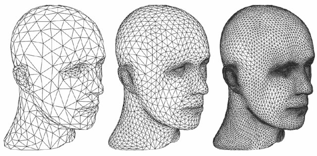
Level Of Detail (Tessellation Parameters)

As the number of triangles used in a trimesh (i.e. its tri-count) increases, the mesh looks more and more like the surface it is approximating. However, the cost of rendering it also increases.

To manage this tradeoff, we often vary a mesh's tri-count based on how much detail we want in the resulting 3D shape. This is loosely expressed as the trimesh's level of detail, which can be captured in the form of one or more tessellation parameters.

**Figure 2:** A face represented by a triangle mesh, at increasing levels of detail.

Single Triangles

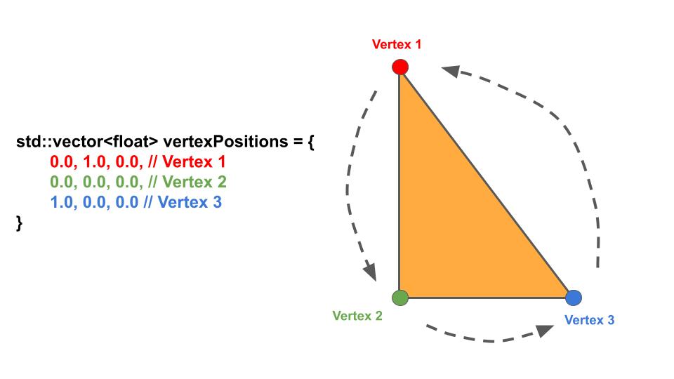
Each triangle in a trimesh is defined by its three vertices, which may have attributes like positions, normals, or colors. First, let's consider only their positions.

Positions

We can store a triangle's vertices' positions in a vector, adopting a counter-clockwise winding order by convention. This simply means that we list the vertices in counter-clockwise order as viewed from the "front" of the triangle.

Normals

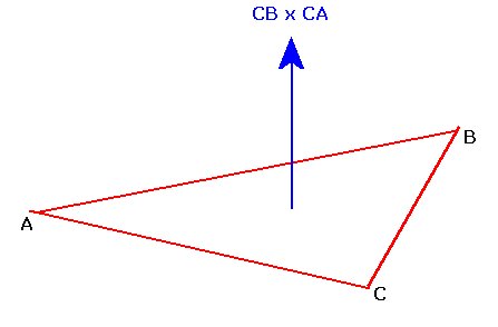
If we're alright with every point on our triangle having the same normal, we can use per-face normals. With three vertices, we can get two vectors; taking the cross product of these gives us the triangle's normal.

**Figure 4:** A triangle's normal can be computed with just its vertices' positions.

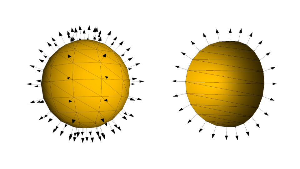
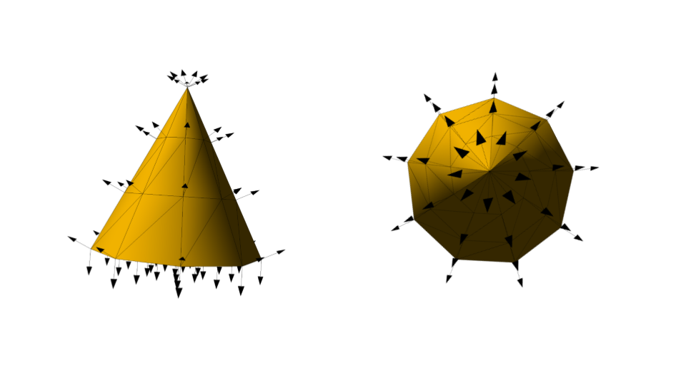
However, we usually want points on our triangle to have different, spatially-varying normals, so that our lighting can (eventually) appear smoother. In such cases, we'd instead use per-vertex normals.

normals on a sphere — **Figure 5:** Per-vertex normals on spheres and cones.

normals on a cone — **Figure 5:** Per-vertex normals on spheres and cones.

For our purposes in CS 1230, we will be using per-vertex normals.

Warning: observe how the tip of the cone in the image above has many normals defined for what appears to be the same vertex. This highlights a critical distinction: by "per-vertex", we don't mean "per-spatial-location", we mean "per-vertex-per-triangle". Many triangles have a vertex located at the tip of the cone, and each of those vertices can have a unique normal.

Positions And Normals

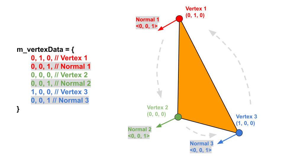
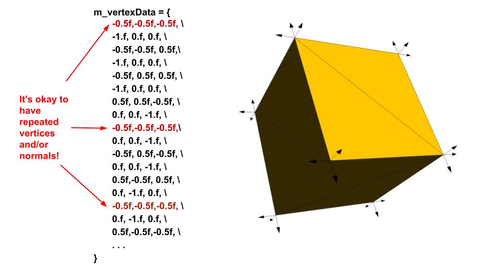
Putting it all together, we can represent each triangle vertex with 6 float values: for its position, and for its normal.

Seeing that each triangle has three vertices, and recalling that we're using a counter-clockwise winding order, we can derive something like m_vertexData below:

Extra: why does winding order matter?

In all subsequent assignments in CS 1230, you will need to use the correct winding order of vertex attributes (e.g. positions and normals) to be able to properly render anything.

This is because, as one of the real-time pipeline's many optimizations, backface culling is enabled by default. This simply means that the "back" faces of each triangle won't be rendered:

**Figure 7:** Backface culling, as seen on a rotating triangle.

Multiple Triangles

To represent a collection of triangles, we simply append the information for each new triangle to the back of our earlier list, i.e.. m_vertexData. Notice that:

Positions and normals are interleaved, just as before; and
Positions might be repeated, which is totally fine—multiple triangles can reasonably share the same position for some of their vertices.

visualization of m_vertexData — **Figure 8:** The vertex data for a cube.

Summary

To summarize the above:

An object can be represented as a number of triangles, varying with its level of detail; and
A collection of triangles can be represented as a list of interleaved positions and normals.

Getting Started

With that out of the way, we're finally at this lab's overarching "super-task":

You will implement three "trimesh generators": one for unit cubes, one for unit spheres, and one for unit cones. These should take in some tessellation parameters, then produce lists of vertex data.

Stencil Code

Take a look at our stencil code. The only files you need to concern yourself with in this lab are Triangle.cpp, Cube.cpp, Sphere.cpp, and Cone.cpp, as well as Tet.cpp for our final debugging exercise. Each of these are located in the src/shapes/ directory.

There is also a Cylinder.cpp file in this directory. You'll want to use this to implement trimeshes for cylinders in Project 5, but you may ignore it for now.

Each shape class contains a member variable std::vector<GLfloat> m_vertexData. Note: a GLFloat is just a float by a different name.

In the body of each shape class' setVertexData() function, you will populate m_vertexData with the positions and normals of your shape's vertices, based on the tessellation parameters provided in m_param1 and m_param2. These tessellation parameters correspond to the parameter sliders in the application window.

The Application Window

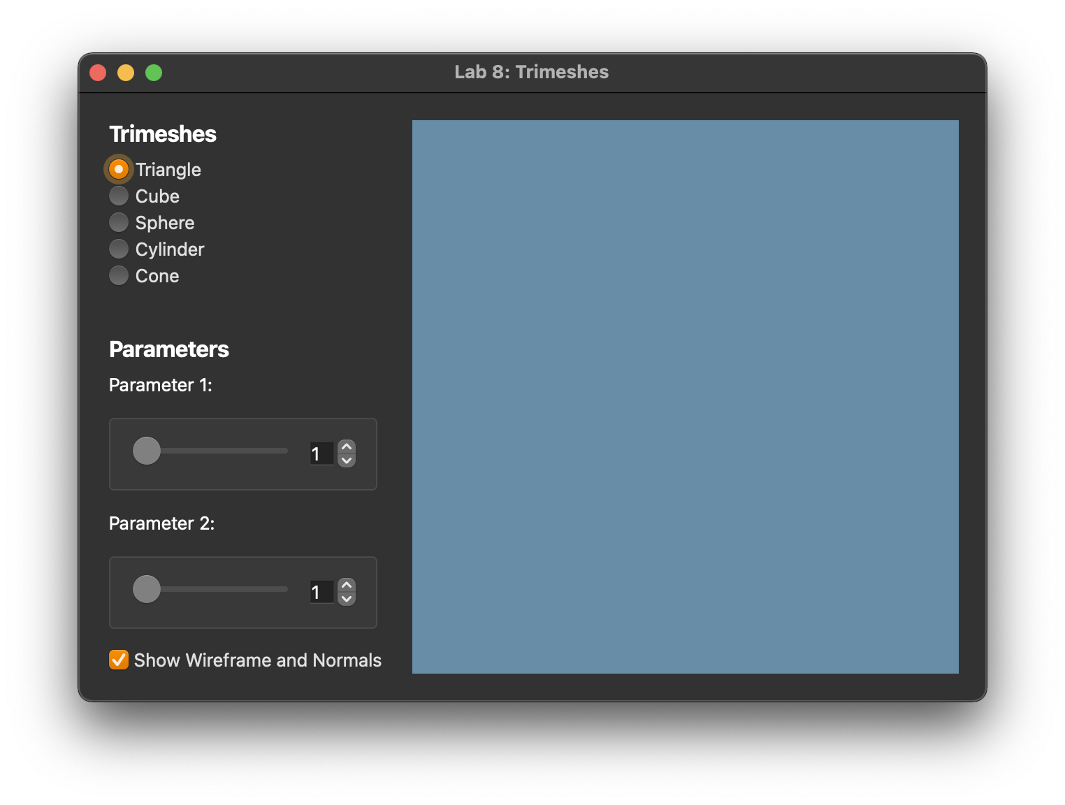
When you first run the program, you'll see a GUI pop-up that looks like this:

On the left sidebar, there are toggles to change the shape and sliders to change tessellation parameters 1 and 2. These control the level of detail of each shape—we'll provide more detail about these later in the handout.

On the right side of the GUI, you will eventually see the shapes generated from m_vertexData. You won't see anything right now because m_vertexData is empty.

Drawing A Triangle

Your first task is draw a triangle to the screen.

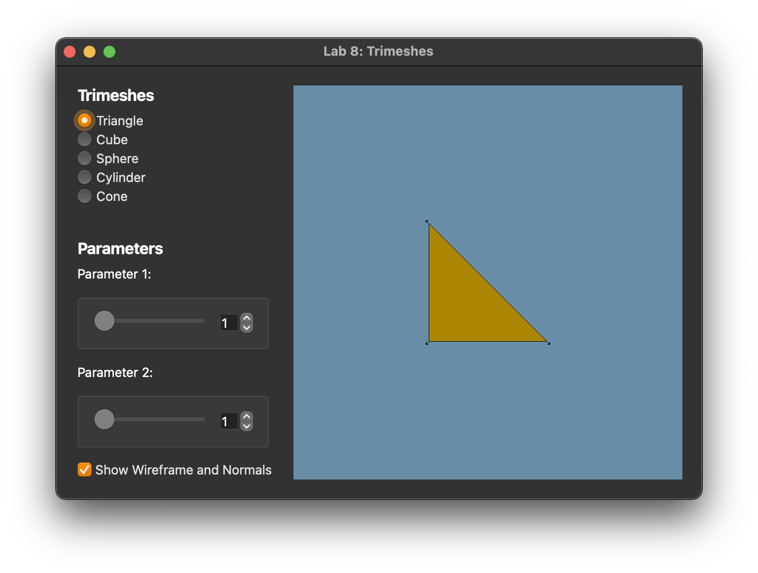
In Triangle.cpp, fill out the setVertexData() function. This function should update m_vertexData with positions and normals. Remember that the normals must be unit vectors.

For your triangle's vertices, please use these positions (listed in no particular order):

(-0.5, 0.5, 0.0)
(-0.5, -0.5, 0.0)
(0.5, -0.5, 0.0)

Which of these positions correspond to which points on the triangle? You don't have to write this one down, but you should be able to answer this question with ease.

Your triangle should look like this:

Observe that if you click and drag to spin the triangle around, it'll disappear at certain angles. This is backface culling! Refer to the dropdown in this section on why winding order matters.

Cubes

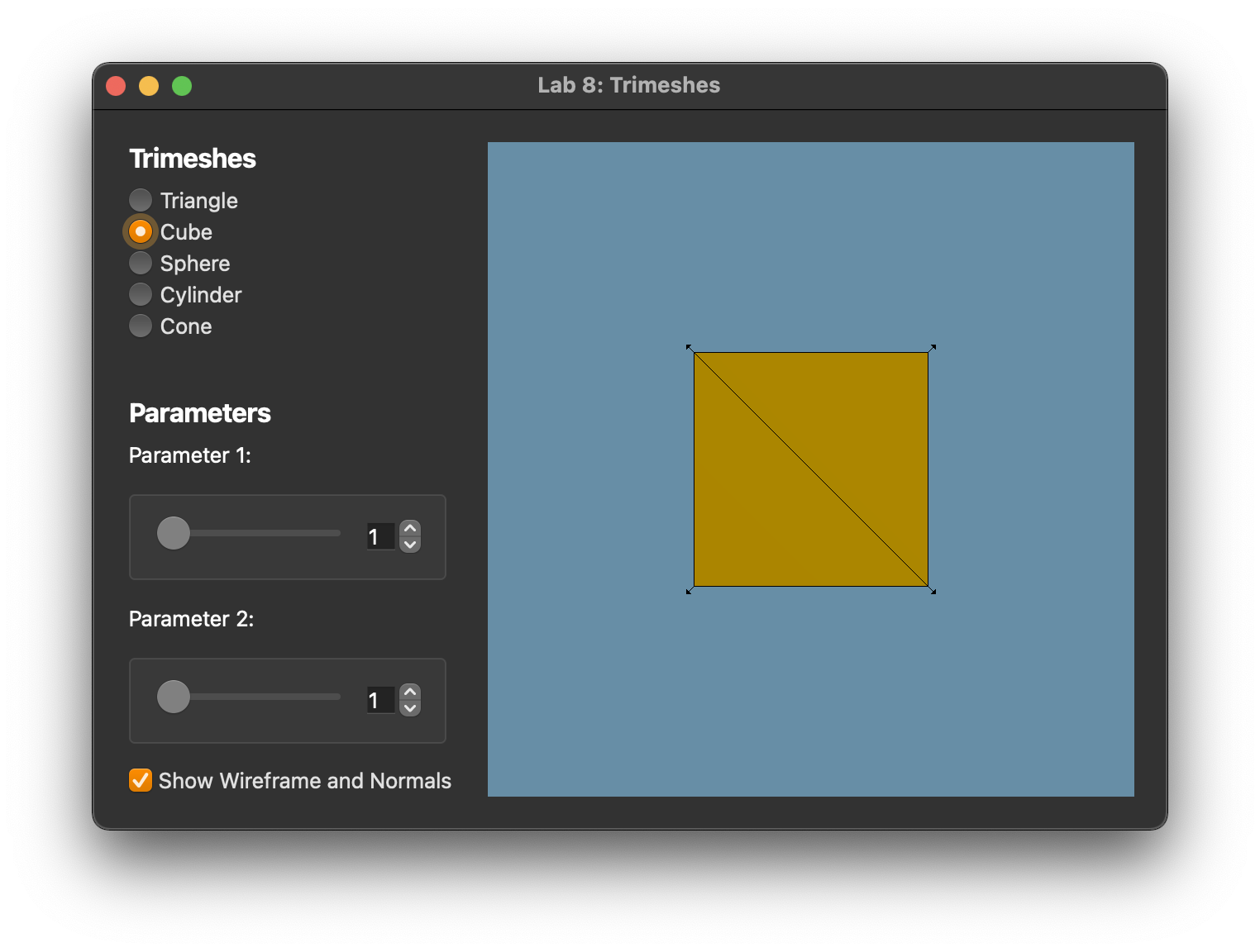
Now that you know how to create a triangle, it's time to render a cube :)

This cube's dimensions are identical to those of the implicit cube from your raytracer. It is centered at the origin, has a side length of 1, and is axis-aligned.

Tiles

To create our cube, you'll first create a "tile": a plane comprising two triangles.

In Cube.cpp:

Uncomment the makeTile() function call in setVertexData().
Implement the makeTile() function. This function should update m_vertexData with a plane made of two triangles created from the input points.
- Use what you learned from making a triangle to do this!
- You will use this function for the next task.

You may find the following glm functions helpful:

glm::vec3 glm::normalize(glm::vec3 v);

glm::vec3 glm::cross(glm::vec3 v1, glm::vec3 v2);

Your tile should look like this:

Cube Faces

Now that you can make individual tiles, you can tessellate a cube face!

Observe how parameter 1 controls the number of tiles in each row and column:

tile parameters — **Figure 12:** Cube faces are increasingly tessellated at higher levels of detail.

In Cube.cpp

Comment out the makeTile() function call in setVertexData() and uncomment the makeFace() function call.
Complete the makeFace() function using the makeTile() function you wrote in the previous task. m_param1 contains the parameter 1 value.

Your face should look like this:

cube face tessellation — **Figure 13:** Expected output of drawing a cube face to the screen, at different levels of detail.

Full Cubes

From here, completing your cube should be a fairly simple task!

Implement the remaining 5 sides of your Cube using the makeFace() function you implemented in the previous task.

It may be helpful to draw a diagram of the Cube to figure out the positions of all its corners!

Your cube should now look like this:

A Cube Tessellating — **Figure 14:** Expected output of drawing a cube to the screen, at different levels of detail

Spheres

Next, we'll set our sights on making a sphere.

This sphere's dimensions are identical to those of the implicit sphere from your raytracer. It is centered at the origin and has a radius of 0.5.

Caught on by now? All the trimesh shapes you'll make have the same dimensions as your implicit ones. This includes the cylinder and cone you'll implement in project 5.

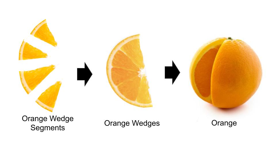
But how do we tessellate a sphere? One way to do so is (bear with us) to think of a sphere like an orange. Oranges are can be sliced into wedges, and each wedge is made up segments. We can therefore build an orange (i.e. a sphere) by procedurally generating a collection of orange wedges.

Extra: this form of sphere tessellation seems familiar to me...

If you've any experience with 3D modelling software like Blender, you'll recognize this to be a UV-sphere, as distinct from an ico-sphere (which is based on subdividing an icosahedron). Here's a pretty good StackExchange discussion about them both.

We use a UV-sphere because it's good enough for our purposes, and it's fairly easy to program. If you're interested in learning about how an ico-sphere is made, you might be interested in searching up different methods for mesh subdivision. Incidentally, Loop subdivision is one of the mesh operations covered in CSCI 2240: Interactive Computer Graphics.

orange anatomy — **Figure 15:** Orange segments make up orange wedges, that in turn make up oranges.

This analogy is helpful for understanding the sphere's tessellation parameters. Parameter 1 controls the number of 'orange segments' (i.e. divisions in latitude), and parameter 2 controls the number of 'orange wedges' (i.e. divisions in longitude).

Refresher: what do latitude and longitude look like, again?

Incidentally, the grid lines in this image show what our sphere will look like, more or less:

lat_long

sphere parameters — **Figure 16:** Spheres faces are increasingly tessellated at higher levels of detail.

Spherical Coordinates

We can represent this 'orange wedge and segment' idea using spherical coordinates. In terms of spherical coordinates, parameter 1 controls and parameter 2 controls .

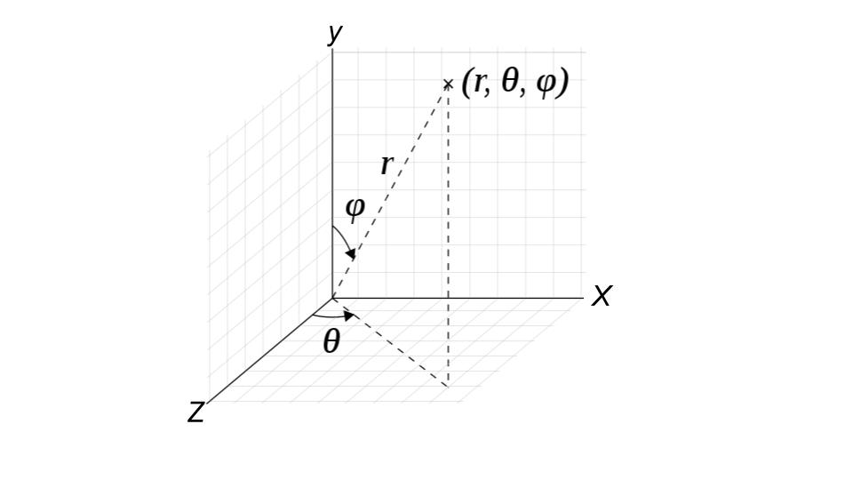
Refresher: the spherical coordinate system

Remember polar coordinates from high school geometry? Spherical coordinates are like polar coordinates, but in 3D, with an added angle of elevation .

The spherical coordinate system thus specifies a 3D point in space using . For more details, please refer to this Wikipedia article on the Spherical Coordinate System.

Wedge

Similar to making a cube, the first step in creating a sphere is to create a tile that can be replicated across the sphere, depending on the level of detail.

In Sphere.cpp, implement the makeTile() function. This function should update m_vertexData.

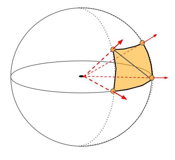
Remember: sphere normals are calculated differently than cube normals.

Figure 18: Sphere normals emanate from the origin.

Once you've implemented makeTile(), you can use it to make a single wedge:

Uncomment the makeWedge() function call in setVertexData().
Implement the makeWedge() function using the makeTile() function you wrote.

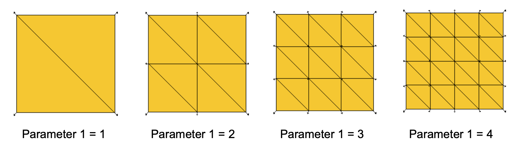
Remember that we are making a wedge, so you need to pay attention to m_param1 and . Refer to the top half of Figure 16 for how m_param1 affects the level of detail. Also note that everything is in radians.

You might find the following functions helpful:

float glm::radians(float x)

float glm::sin(float x)

float glm::cos(float x)

You might also find these equations useful:

x = r * sin(phi) * cos(theta)

y = r * cos(phi)

z = -r * sin(phi) * sin(theta)

Your single wedge should look like this:

wedge tessellating — **Figure 19:** Expected output of drawing a wedge to the screen, at different levels of detail.

Full Spheres

We can now use our makeWedge() function to generate a full sphere!

Comment out the makeWedge() function call in setVertexData() and uncomment the makeSphere() function call.
Implement the makeSphere() function using makeWedge().

Remember that we are making multiple wedges (i.e. a sphere), so you need to pay attention to m_param2 and . Refer to the bottom half of Figure 16 for how m_param2 affects the level of detail.

Your sphere should look like this:

Completed Sphere — **Figure 20:** Expected output of drawing a sphere to the screen, at different levels of detail.

Cones

Finally, we'd like to render a cone.

When rendering a cone, instead of using spherical coordinates, we only need to specify angle in the horizontal plane. This means that instead of specifying points using as in spherical coordinates, we substitute out for a Cartesian -coordinate.

This new coordinate system is known as the cylindrical coordinate system. For more info, refer to this Wikipedia article on the Cylindrical Coordinate System.

Wedges

Just like our sphere, we can divide this cone into wedges, where parameter 2 represents the number of total wedges.

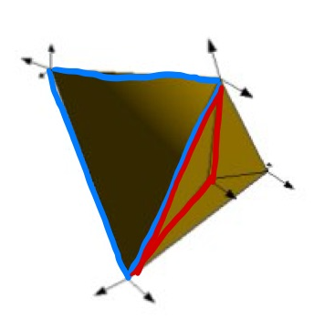
However, these are different from sphere wedges, as they consist of two independent components: a slope slice and a cap slice. See the diagram below for what this looks like.

Cone Wedge — **Figure 3:** One wedge of a cone. The blue triangle is the slope slice, and the red triangle is the cap slice.

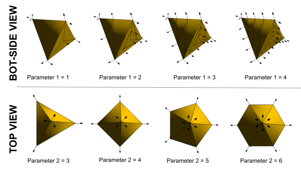
Importantly, both the slope slice and cap slice components need to be subdivided. Parameter 1 represents the number of rectangular tiles each is subdivided into. (Note that in both types of components, one rectangular tile will look like a triangle as one of its constituent triangles has zero area.)

Put together, here are some views of a tessellated cone with different parameters:

**Figure 3:** Tessellated Cone Parameters

Cap Slice

First, let's build and triangulate a cap slice:

In Cone.cpp, implement the makeCapSlice() function. We strongly recommend you make a helper function makeCapTile() that adds an individual tile to m_vertexData.

You might find these equations useful to convert from cylindrical to rectangular coordinates:

x = r * cos(theta)

z = r * sin(theta)

Slope Slice

Next, let's build and triangulate a slope slice.

In Cone.cpp, implement the makeSlopeSlice() function. Similarly to above, you probably want to make a helper function makeSlopeTile().

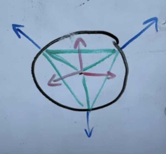
Just like we did for our sphere, we want to use slope normals for the actual implicit cone (not our trimesh cone). This formula is a little more complex, so we'll provide it for you here:

glm::vec3 Cone::calcNorm(glm::vec3& pt) {
    float xNorm = (2 * pt.x);
    float yNorm = -(1.f/4.f) * (2.f * pt.y - 1.f);
    float zNorm = (2 * pt.z);

    return glm::normalize(glm::vec3{ xNorm, yNorm, zNorm });
}

Why does this work?

Take some triangular cross-section of the cone that passes through its center axis. Let be the radius of the base (half the base in the cross section). What is the 2D slope of one of the slope faces?

Before normalizing, suppose the horizontal component of the normal has magnitude . What should the -component of the normal be?

You'll also have to consider the edge case of calculating normals for the tip of the cone.

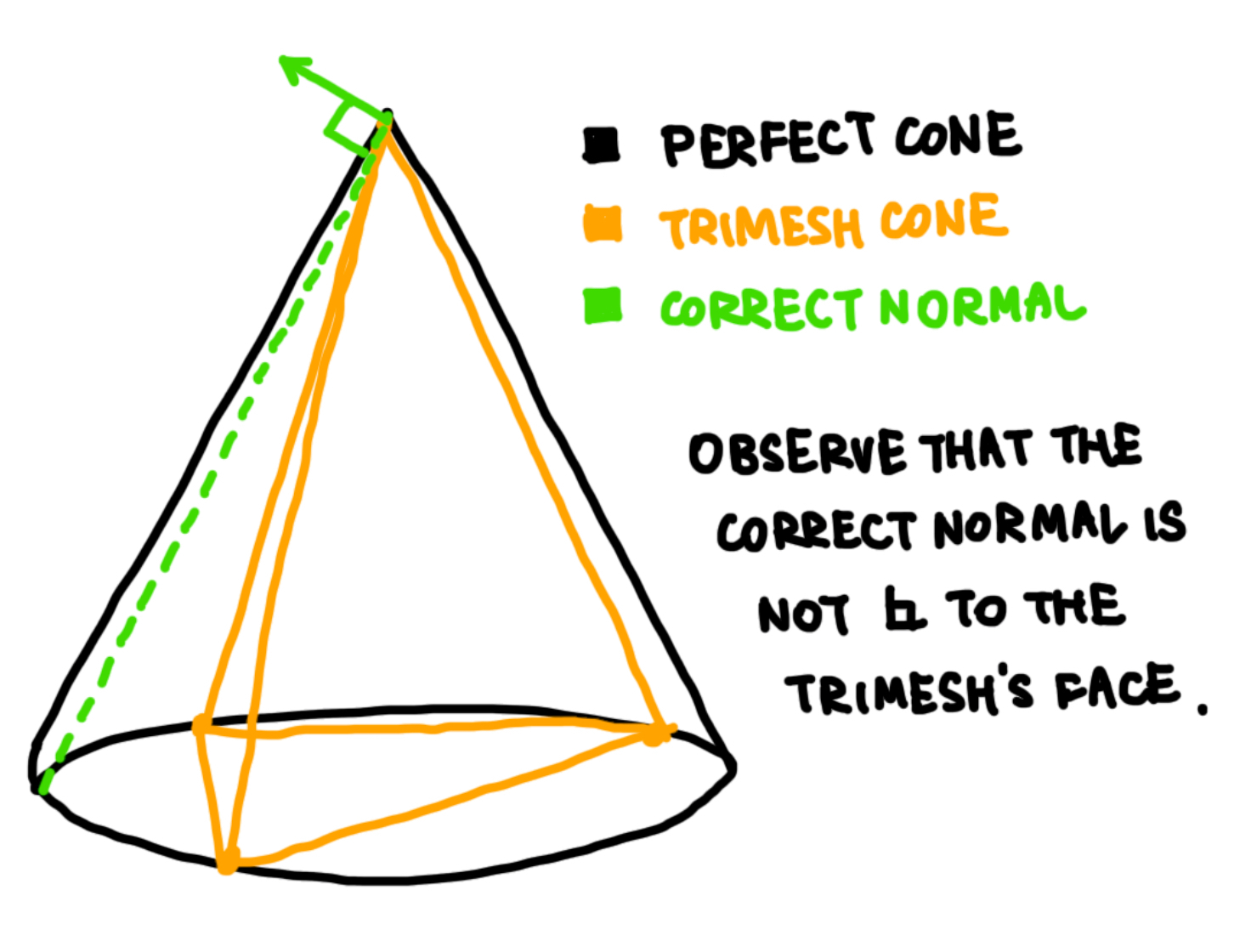
At the cone tip, we still want the normal to be perpendicular to the implicit cone (not our trimesh cone), BUT we want the horizontal component to be in the direction of each slope face (instead of each slope edge, as you might expect).

TODO: FIX FIGURE NUMBERS

Correct Cone Tip Normal Diagram

Cone Tip Normals Special Case — **Figure 4.5:** Correct cone tip normal that is align with that of an implicit cone. Note that the normal is located half-way radially between the edge normals.

Hint about cone tip normal calculation

One valid approach to calculating normals at the cone tip is to take the average of the two normals of the base triangle (remember to normalize it afterwards!).

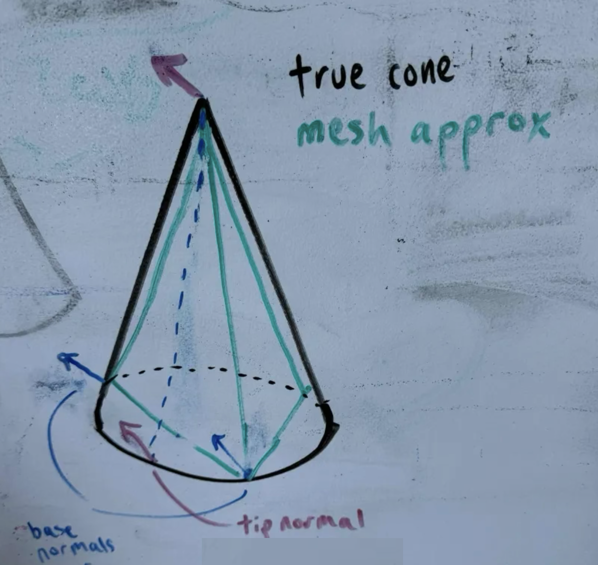
More detailed explanation:

Cone Top-Down Diagram — **Figure 4.6:** Top-down view of the implicit cone and its mesh approximation. Red indicates the true tip normal and blue indicates the face normal at the top of the corresponding mesh face.

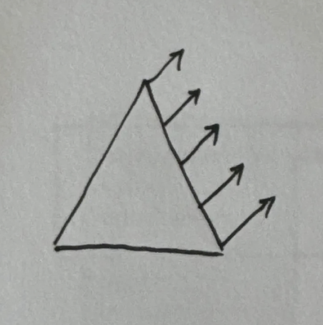
Figure 4.6 shows that the cone tip normal lies halfway between the two face normals at the top of the corresponding mesh face. If we were to take a vertical slice of the cone, we would see that the normals all point in the same direction along the surface, going up that slice:

Vertical Slice of Cone — **Figure 4.7:** Vertical slice of a cone.

This means that the two base normals of that face are the same as the two normals at the top of the face, so the cone tip normal can be found by taking the average of the base normals.

Cone Tip Normals — **Figure 4.8:** Final diagram showing base normals and cone tip normal.

Full Cones

Now we're ready to generate a full cone!

Fill out the makeWedge() function that uses makeCapSlice() and makeSlopeSlice() to make one wedge of a cone.
Using makeWedge(), fill in the logic for rendering an entire cone in setVertexData().

Debugging

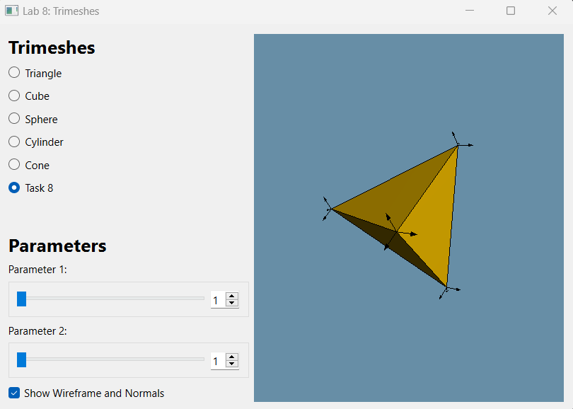
Finally, as a quick exercise in debugging visually, we've provided you with a buggy tesselation of a tetrahedron with vertices ABCD in Tet.cpp. The geometry of the tetrahedron has no issues, but its shading looks a little off. It's your task to identify and correct the issue in setVertexData().

In the GUI, select Task 8 to display the shape. Use your mouse to rotate the tetrahedron to see all its sides.

Notice that one of the triangles (triangle ADB in the code) appears dark, even when it faces the light source behind the camera.

gif of the buggy and expected tetrahedrons. — **Figure 21:** Buggy vs. Expected lighting of the tetrahedron.

Fix the bug in setVertexData() in Tet.cpp!

Click for hints:

We should expect triangles that directly face the light to appear brighter vs. ones that face away from the light, because the term of the diffuse lighting component is largest when (the surface normal) aligns with (the direction from the surface to the light). This suggests that something might be wrong with the normals, which are used to compute lighting.
Recall that each triangle has a unique orientation determined by its vertex ordering. By convention, the direction of the normal depends on the right hand rule. So, the normal of a triangle can be determined by the cross product , where is the vector from to , and similarly for . See the diagram in figure 4 for another equivalent example.

You only need to consider the code in lines 8 to 27 of Tetrahedron::setVertexData().

While it's often tempting to dive straight into debugging code when you encounter issues, learning to debug visually is a crucial skill in computer graphics. Identifying high-level problems with the outputs of your programs can help you quickly narrow down potential low-level causes in your code.

End

Congrats on finishing the Trimeshes lab! Now, it's time to submit your code and get checked off by a TA.

Submission

Submit your GitHub link and commit ID to the "Lab 8: Trimeshes" assignment on Gradescope, then get checked off by a TA at hours.

Reference the GitHub + Gradescope Guide here.