Project 4: Antialias

Github Classroom assignment (same assignment as before)

You can find the section handout for this project here.

Introduction

By now, you have a powerful ray tracer in your hands, able to produce beautiful renders complete with shadows, textures, and even recursive reflections! At some point though, something may have bothered you about the produced images.

Often referred to as “jaggies”, this is an instance of the signal processing phenomenon known as aliasing. In this case, our ray tracer is not sufficiently sampling these object silhouettes, causing an implicitly smooth edge to appear in (i.e. alias to) a jagged, stair-step pattern.

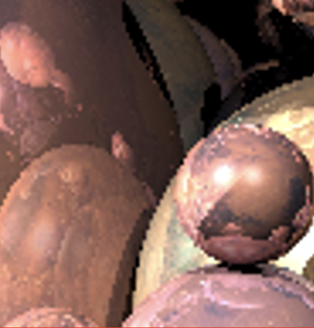
Aliasing can also occur on textured objects, like this:

Requirements

For this project, you will incorporate the following antialiasing techniques into your ray tracer:

Supersampling

Super-sampling aims to mitigate aliasing by sampling each pixel at multiple locations. This leads us to two questions: Where should we sample from? How many samples should we use?

Regular Grid Sampling

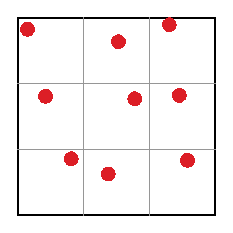
The simplest approach is to sample the pixel in a regular grid pattern. For example, if we want to take 9 samples per pixel, we can sample at the centers of each cell of a 3x3 grid, like this:

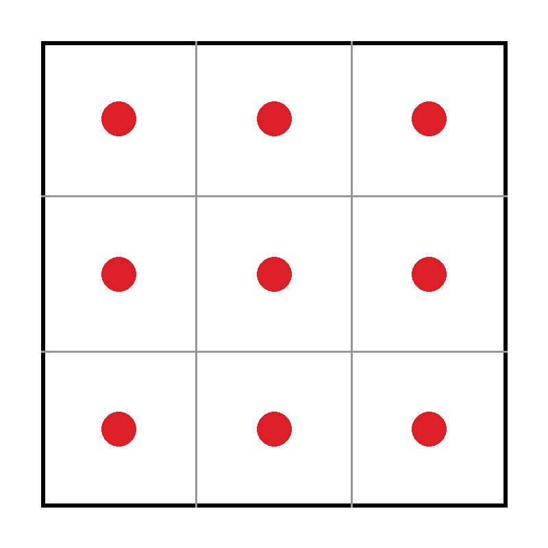
For this assignment, we only expect you to implement square sampling patterns (e.g. 1, 4, 9, 16, samples per pixel). If the .ini file for your scene specifies a non-square number of samples per pixel, it is fine to round up to the nearest square. However, you are welcome to experiment with other patterns, if you wish.

Random Sampling

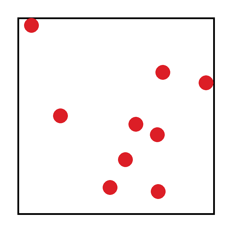
Regular grid sampling can lead to artifacts, since the sampling pattern is correlated with the pixel grid. An alternative is to sample uniformly at random within the pixel, like this:

Think about how you might produce such a uniform random sampling pattern. You're welcome to use any random number generation library you like, such as the C++ standard library's <random> header.

Stratified Sampling

Random sampling trades off potential grid-based artifacts for noise. But purely random samples can be quite clumpy: some areas of the pixel are oversampled while others are undersampled, leading to more noise. Stratified sampling attempts to mitigate this problem by combining regular grid sampling with random sampling: it divides the pixel into a grid and takes one random sample within each grid cell. For example, if we want to take 9 samples per pixel, we can divide the pixel into a 3x3 grid, and take one random sample within each grid cell, like this:

As with regular grid sampling, it is fine to round up to the nearest square number of samples per pixel if the .ini file specifies a non-square number.

Adaptive Sampling (Extra Credit)

You may notice that your runtime has significantly increased after implementing supersampling, since you're tracing many more rays per pixel. You may also notice that you start getting diminishing returns from increasing the sampling rate: many pixels do just fine with 1-4 samples per pixel, and the more samples you add, the fewer pixels benefit from each added sample.

This observation suggests an optimization: we can adaptively choose how many samples to take per pixel, based on how much variation there is between samples in the pixel. For example, if a pixel covers a constant-color patch of the scene, we can probably get away with taking only 1 sample. But if a pixel falls on an edge or a patch of high-frequency texture, we may want to take more samples.

There are many ways to implement adaptive sampling. One simple approach is to take a small number of initial samples (e.g. 4), and compute the statistical variance of those samples. If the variance is below some threshold, we can stop and use the average of those samples as the pixel color. If the variance is above the threshold, we can take more samples (e.g. 4 more), and repeat the process until we reach a maximum number of samples per pixel.

Texture Filtering

Supersampling attempts to sample the image at a high enough rate that aliases don't occur. But this is expensive, and sometimes its impossible (e.g sharp edges that introduce infinite frequency content). An alternate strategy is to get rid of frequency content in the image that we can't reprsent with our sample budget. That's hard to do in general, but it is (approximately) possible for textures.

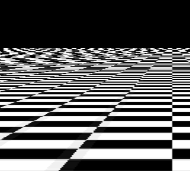
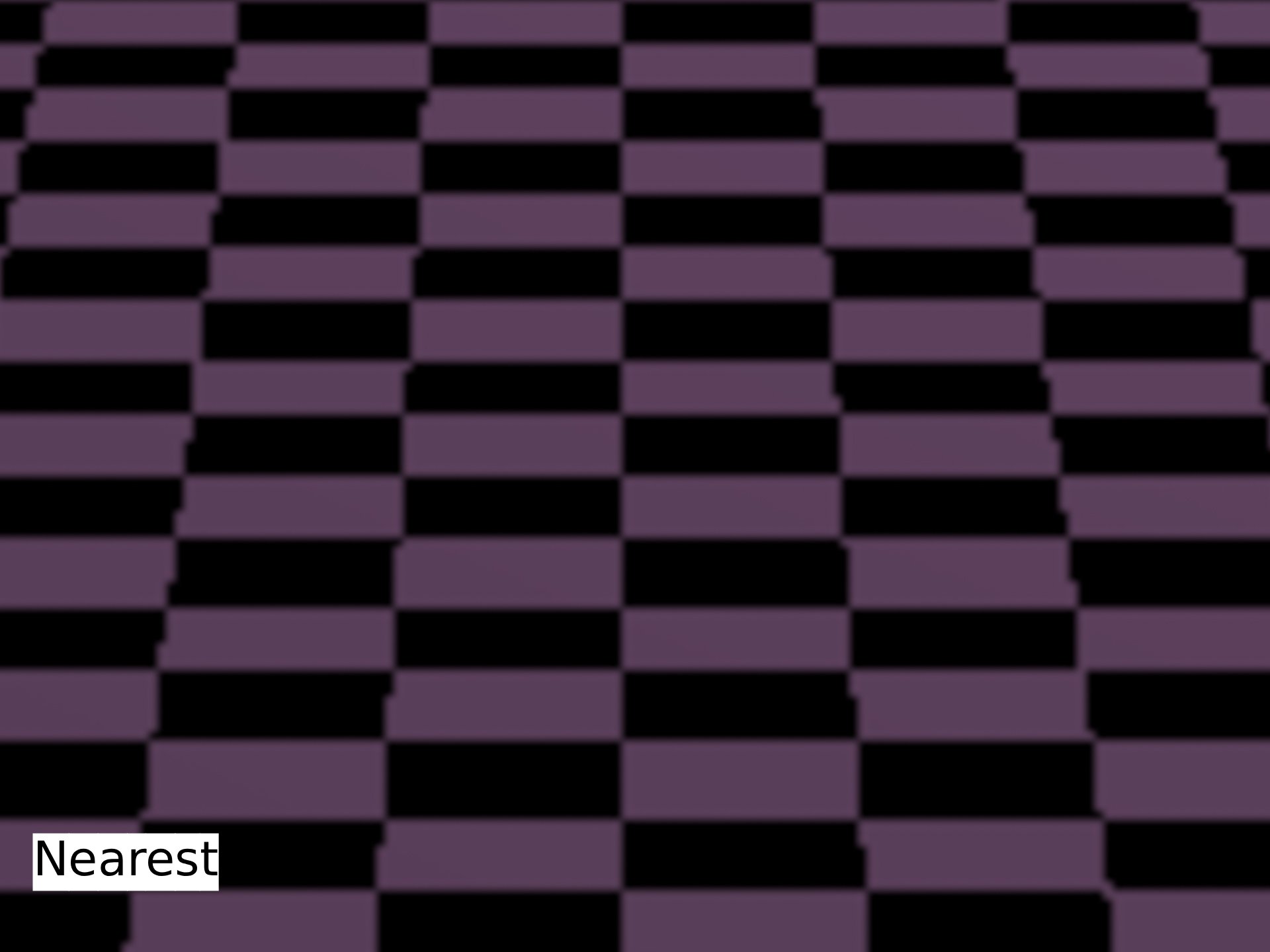
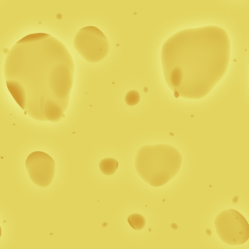
In the previous project, when you looked up the texture value at an intersection point, you retrieved the texel (texture map pixel) that was closest to the intersection point. This is called nearest-neighbor sampling, and it can lead to aliasing artifacts when the texture is viewed at a distance or at a steep angle. For example:

In this project, you'll implement some better texture sampling techniques to reduce these artifacts.

Bilinear Filtering

Bilinear filtering is a simple improvement over nearest-neighbor sampling. Instead of just taking the value of the nearest texel, we take a weighted average of the 4 nearest texels. This is equivalent to filtering the texture with a 2x2 triangle filter. Doing so results in improved image quality, like this:

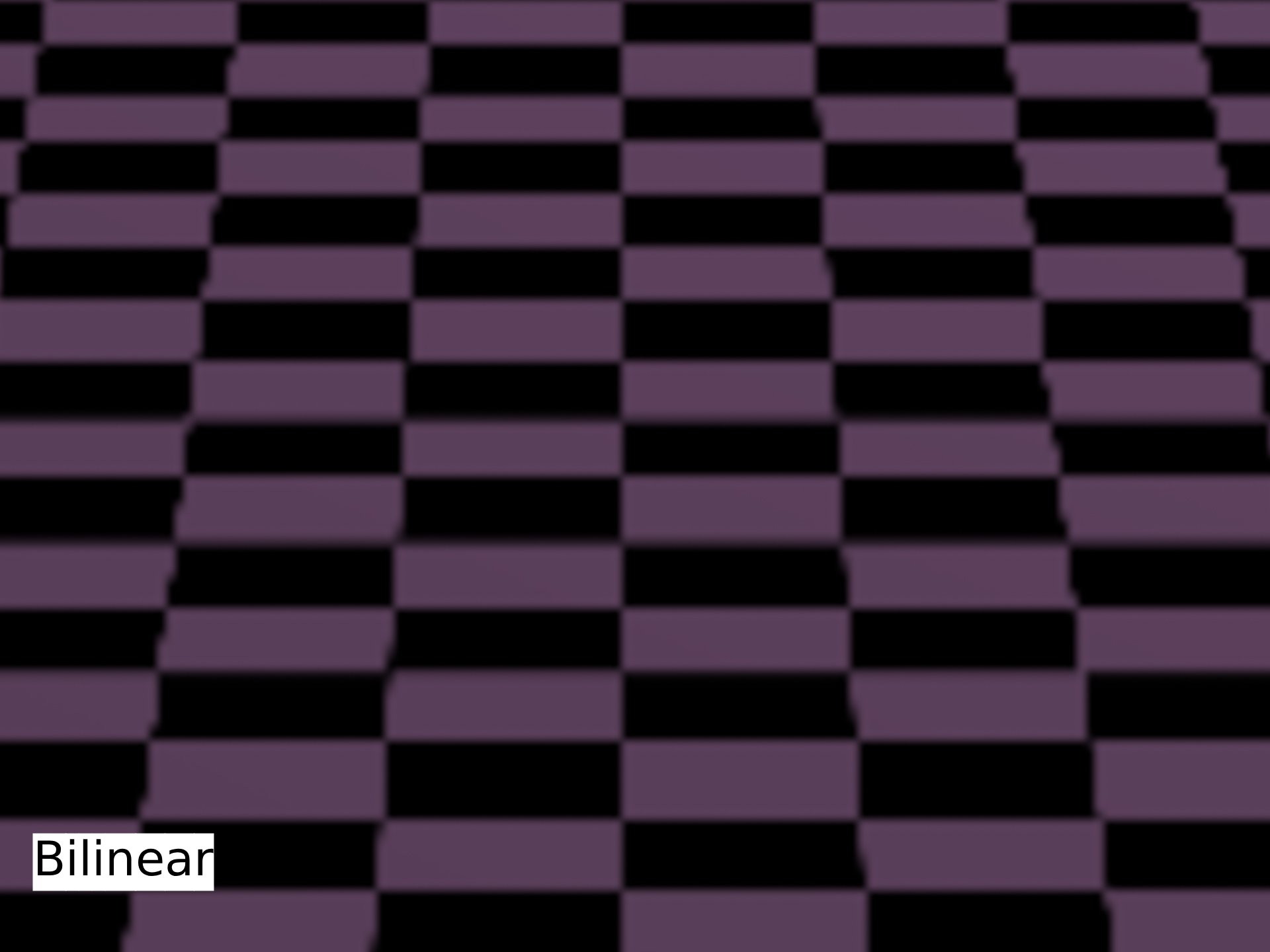
Here is the difference between the two:

Mipmapping

Bilinear filtering helps, but a fixed 2x2 filter window is not always enough. When a texture is viewed at a steep angle or from a distance, a pixel may cover many texels. In this case, we should be averaging over a larger area of the texture to minimize aliasing. Ideally, we would filter the texture with a filter whose size is proportional to the pixel's footprint on the texture. However, doing so would be prohibitively expensive at render time. Instead, we can precompute a series of downsampled versions of the texture, called mipmaps (short for "multum in parvo", Latin for "many things in a small place"). Each level of the mipmap is downsampled by a factor of 2 in each dimension. Then, at render time, we can choose the appropriate mipmap level(s) to sample from based on a pixel's footprint on the texture.

Implementing mipmapping requires multiple steps, which we outline below.

Downsampling

Generating mipmaps requires the ability to properly downsample an image. Thus, you'll need to implement a function that can take an image and scale it down by an artbitrary factor, being sure to use a pre-filter which avoids introducing aliases. You should use a triangle filter for this purpose (though you can use better filters for extra credit), and you should implement it as a separable filter for efficiency. Everything you need to know for this implementation has already been covered in great depth during the Sampling, reconstruction, & antialiasing lectures.

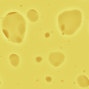
Here's an example of downsampling an image by a factor of 4 using a triangle filter:

Mipmap Generation

Once you've implemented downsampling, you can generate mipmaps for every texture in your scene.

• You should generate mipmaps during scene loading, so that you don't have to pay the cost of generating mipmaps at render time. In fact, you will lose efficiency points if you generate mipmaps at render time.
• For each texture, generate all possible mipmap levels, starting at the original image size and going all the way down to a 1x1 image.
• Since we're doing offline rendering, we can trade some speed for quality. Thus, you should produce each mipmap level by downsampling from the original image, rather than downsampling the previous mipmap level by a factor of 2.

Think about the way you'll use these downscaled images in your raytracer, and choose an appropriate data structure to keep track of them.

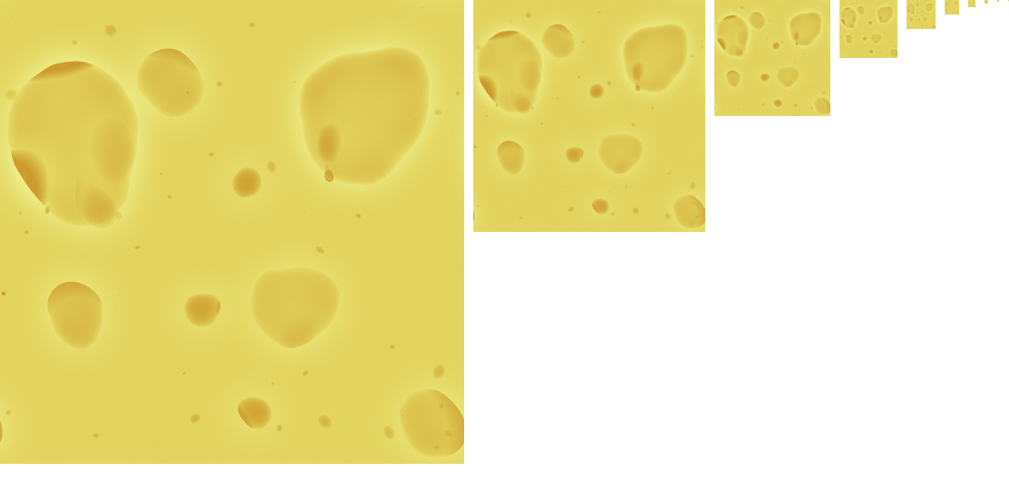
Here's an example of what a mipmap pyramid (i.e. the set of all mipmap levels for a given texture) might look like:

Determining Mipmap Level at Render Time

When you sample from a mipmapped texture, you should determine which mip level to sample from. To do that, you must determine the pixel's “footprint” upon the texture, i.e. how many texels are covered by the screen pixel through which the current ray was traced. In lecture, we discussed how to do this using a bit of differential calculus; you'll need to implement that approach here.

Recall that one of the steps in this process involves computing the derivatives of the surface coordinates with respect to the object space intersection point . In algo section, you'll work through the math to compute these derivatives for spheres. In this project, you'll need to figure out the implementation of the corresponding derivatives for the other types of primitives supported by your raytracer (cubes, cones, and cylinders). You are welcome to use external resources to help you, provided you cite them in your submission. You might find online symbolic math calculators such as Wolfram Alpha or Symbolab helpful for working through the math.

Trilinear Filtering

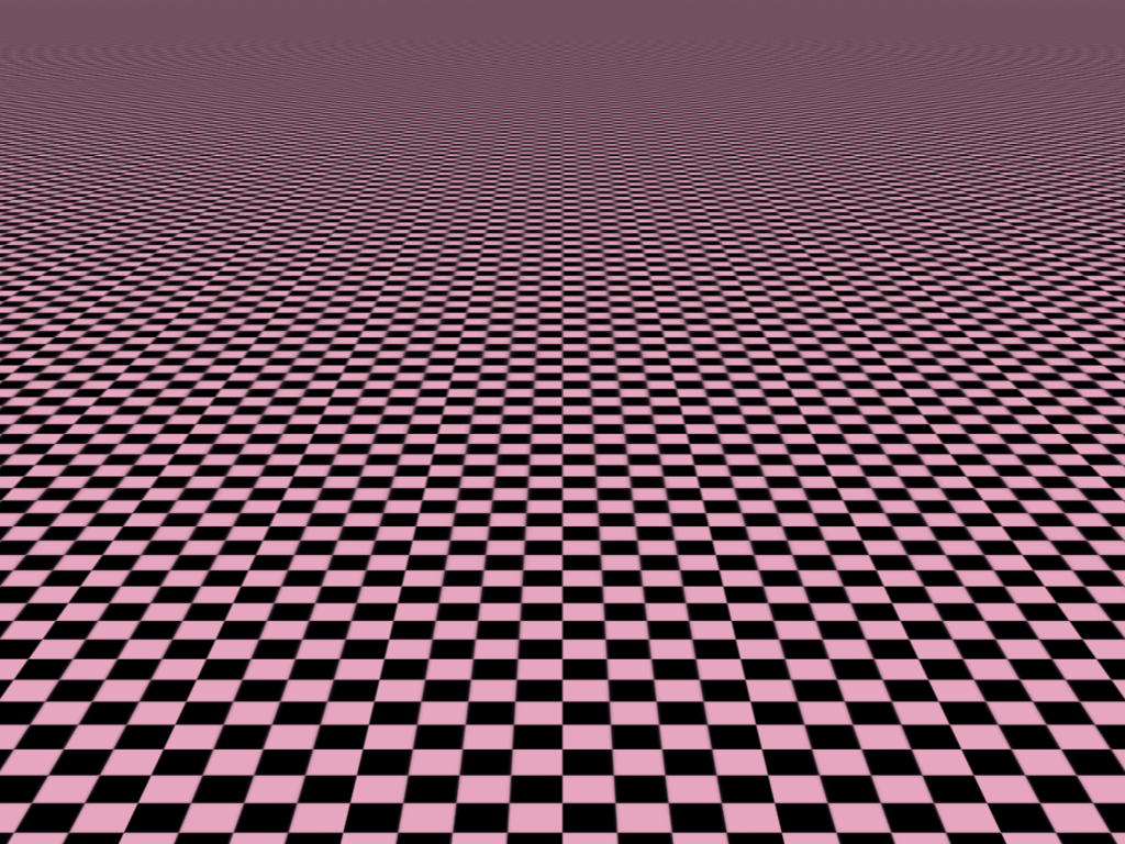
One downside of using a single mipmap level is that the transition between levels can be abrupt, leading to noticeable 'seam' artifacts. For example, here's the checkerboard floor scene from earlier, rendered with bilinear filtering and a single mipmap level:

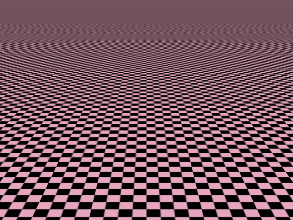
We can eliminate these artifacts by instead interpolating between two adjacent mipmap levels. This is called trilinear filtering, since it involves bilinear filtering in the two spatial dimensions, plus linear interpolation between the two mipmap levels.

When you compute the footprint of a pixel on the texture (based on the equations from lecture), you get a value in units of texels; taking the base 2 logarithm of that value gives you a floating point mipmap level. The integer part of that value tells you which two mipmap levels to interpolate between, and the fractional part tells you how to weight the two levels. For example, if the computed mipmap level is 3.2, you would bilinearly filter from mipmap levels 3 and 4, and weight them 0.8 and 0.2, respectively.

Here's the improvement you can expect from trilinear filtering:

GLM Library Functions

Please avoid using the following GLM functions, as we have covered how to implement them in class:

• glm::lookAt(eye, center, up)

• glm::reflect(I, N)

• glm::perspective(fovy, aspect, near, far)

• glm::mix(x, y, a)

• glm::distance(p1, p2)

Codebase & Design

Your work on this project will extend your code from the Intersect and Illuminate projects; there is no additional stencil code.

As before, the structure of this project is entirely up to you: you can add new classes, files, etc. However, you should not alter any command line interfaces we have implemented in the code base.

We provide all the rendered results of the scenes we have in the scenefiles folder under antialias/required_outputs, antialias/optional_outputs, and antialias/extra_credit_outputs. They serve as references for you to check the correctness of your implementation.

sh run-antialias.sh

Scenes Viewer

To assist with creating and modifying scene files, we have made a web viewer called Scenes. From this site, you are able to upload scenefiles or start from a template, modify properties, then download the scene JSON to render with your raytracer.

We hope that this is a fun and helpful tool as you implement the rest of the projects in the course which all use this scenefile format!

For more information, here is our published documentation for the JSON scenefile format and a tutorial for using Scenes.

TA Demos

Demos of the TA solution are available in this Google Drive folder.

Instructions for Running

You can run the app from the command line with the same .ini filepath argument that you would use in QtCreator. You must put the executable inside of your build folder for this project in order to load the scenefiles correctly.

On Mac:

open projects_antialias_<min/max>.app --args </absolute/filepath.ini>

On Windows and Linux:

./projects_antialias_<min/max> </absolute/filepath.ini>

Grading

This assignment is out of 100 points.

• Supersampling
  • Regular Grid Sampling (5 points)
  • Random Sampling (4 points)
  • Stratified Sampling (6 points)
• Texture filtering
  • Bilinear Filtering (10 points)
  • Image Downsampling (25 points)
  • Mip-map Generation (5 points)
  • Determining Mip-map Levels (20 points)
  • Trilinear Filtering (5 points)
• Software engineering, efficiency, & stability (20 points)

Extra Credit

All of the extra credit options from Intersect or Illuminate are also valid options here (provided you haven't already done them). In addition, you can consider the following options (or come up with your own ideas):

• Cache pre-computed mipmaps (3 points): Develop a scheme to save your mipmaps to disk and re-use them when rendering the same scene multiple times (e.g. from different camera angles)
• Adaptive supersampling (up to 5 points): In the Adaptive Sampling section above, we described one possible approach to adaptive sampling. You are welcome to implement that approach, or come up with your own.
• Quasi-Monte Carlo sampling (up to 5 points): Implement a low-discrepancy sampling pattern (e.g. Halton, Hammersley, or Sobol sequences) for supersampling.
• Better pre-filtering for mipmap generation (up to 4 points): Use a better filter than a triangle filter for downsampling when generating mipmaps. You can use a Gaussian filter, a Lanczos filter, or any other filter of your choice.
• Better filtering for render-time texture sampling (up to 4 points): When sampling a value from a given mipmap level, use a better filter than bilinear filtering. You can use bicubic filtering, a Gaussian filter, or any other filter of your choice.
• Anisotropic filtering (up to 15 points): Implement a method for anisotropic (i.e. direction-varying) texture filtering. Ripmaps, summed-area tables, and mipmap multisampling are all described briefly in Section 5.2 of this book chapter. Elliptical weighted averaging (EWA) is often considered the "gold standard" for anisotropic texture filtering. It is hard to find a good reference for it; these slides introduce it at a high-level, and the approach was originally introduced in Paul Heckbert's masters thesis (Section 3.5.8).
• Full ray differentials (10 points): Implement tracking of ray differentials for correct ray footprint determination through reflections (and refractions, if you implemented that as extra credit in the previous project). The original paper on ray differentials is a helpful reference.
• Cone tracing: Cone tracing is a geometry-based (as opposed to calculus-based) approach to determining ray footprints. Section 20.3.4 of this book chapter provides a good reference.
  • Cone tracing for eye rays (up 5 points)
  • Cone tracing for eye rays & recursive rays (up to 15 points)

Tips & Hints

• When implementing mipmapping, we highly recommend that you visualize the mipmap levels you are generating to ensure that they look sensible (i.e. like downsampled versions of the original texture). If you store your mipmaps as QImages, you can easily save them to disk using QImage::save(filename), where filename is a string containing the path to the file you want to save to. You can use a naming scheme like texture_mip_0.png, texture_mip_1.png, etc. to keep track of the different levels.
• A good way to check whether your ray footprint calculation (and thus mipmap level determination) is working correctly is to color ray intersections by mipmap level. For example, you can set the color of an intersection to be a grayscale value between and , where is the mipmap level used for that intersection, and is the maximum mipmap level for that texture.

Milestones

Although how you approach the steps of the project is entirely up to you, we have provided a rough milestone of steps to help you code incrementally. Since this is a just an outline, please double check the submission requirements to ensure you have completed all necessary functionalities.

Week 1:

• Implement supersampling (regular grid, random, and stratified)
• Think about how you plan to implement mipmapping (e.g. where each of the parts of the implementation will go in your codebase, what data structures you'll use to store mipmaps, how the interfaces to your existing code will change, etc.)
• Implement bilinear filtering for texture sampling.
• Start working on image downsampling. This is the biggest single chunk of work in the whole project, so don't save it until the last minute!

Week 2:

• Finish image downsampling
• Implement mipmap generation
• Implement determining mipmap levels at render time for eye rays
• Implement trilinear filtering

Submission

Submit your GitHub repo and commit ID for this project to the "Project 4: Antialias" assignment on Gradescope.

Your repo should include a submission template file in Markdown format with the filename submission-antialias.md. We provide the exact scenefiles you should use to generate the outputs. You should also list some basic information about your design choices, the names of students you collaborated with, any known bugs, and the extra credit you've implemented.

For extra credit, please describe what you've done and point out the related part of your code. If you implement any extra features that requires you to add a parameter for QSettings.ini and RayTracer::Config, please also document it accordingly so that the TAs won't miss anything when grading your assignment. You must also include test cases (usually, videos or images in the style of the output comparison section) that demonstrate your extra credit features.

Please let us know if you find any mistakes, inconsistencies, or confusing language in this or any other CS 1230 document by filling out our anonymous feedback form.